K近邻(K-Nearest Neighbor,KNN)算法是一种基本分类与回归方法,也是最简单的机器学习方法之一,这里只对K近邻算法的分类问题做总结。
K近邻算法简单、直观,它的工作原理是:给定一个训练数据集,对新的输入实例,在训练数据集中找到与该实例最近邻的(k)个实例,这(k)个实例的多数属于某个类,就把该输入实例分为这个类。
1 K近邻模型的基本要素
K近邻模型的三个基本要素——距离度量、(k)值的选择和分类决策规则
1.1 距离度量
特征空间中两个实例点的距离反映两个实例点的相似程度。(k)近邻模型的特征空间一般是(n)维实数向量空间(R^n),使用的距离是欧式距离,但也可以是其他距离。
在特征空间中取两个特征(x_i),(x_j),它们都是(n)维向量。(x_i),(x_j)的(L_p)距离定义为
其中(p≥1)。当(p=2)时,称为欧式距离
当(p=1)时,称为曼哈顿距离
1.2 (k)值的选择
(k)值的选择对(k)近邻算法的结果影响重大。选择较小的k值,就相当于用较小的领域中的训练实例进行预测,训练误差会减小,只有与输入实例较近或相似的训练实例才会对预测结果起作用,与此同时带来的问题是泛化误差会增大。换句话说,k值的减小就意味着整体模型变得复杂,容易发生过拟合。选择较大的k值,就相当于用较大领域中的训练实例进行预测,其优点是可以减少泛化误差,但缺点是训练误差会增大。这时候,与输入实例较远(不相似的)训练实例也会对预测器作用,使预测发生错误。换句话说,k值的增大就意味着整体的模型变得简单,容易发生欠拟合。
在应用中,(k)值一般取一个比较小的数值,通常采用交叉验证法来选取最优的(k)值。
1.3 分类决策规则
(k)近邻算法中的分类决策规则往往是多数表决。
2 K近邻算法的代数方式描述
输入:训练数据集
其中,(x_{i}epsilon chi subseteq R^{n})为实例的特征向量,(y_{i}epsilon left { c_{1},c_{2},cdot cdot cdot ,c_{K}
ight })为实例的类别,(i= 1,2,cdot cdot cdot ,N);实例特征向量(x);
输出:实例(x)所属的类(y).
(1)根据给定的距离度量方式,在训练集T中找到与(x)最邻近的(k)个点,涵盖着(k)个点的(x)的领域记作(N_{k}left ( x
ight ));
(2)在(N_{k}left ( x
ight ))中根据分类决策规则决定(x)的类别(y):
其中(I)为指示函数,即当(y_{i}=c_{j})时(I)为1,否则(I)为0
from numpy import*  #NumPy科学计算包
import operator  #运算符模块

#创建数据集和标签
def createDataSet():
    group = array([[1.0, 1.1], [1.0, 1.0], [0, 0], [0, 0.1]])
    labels = ['A', 'A', 'B', 'B']
    return group, labels

group, labels = createDataSet()
group, labels
#输出
[[ 1.   1.1]
[ 1.   1. ]
[ 0.   0. ]
[ 0.   0.1]] ['A', 'A', 'B', 'B']
3.2 实施KNN算法
对未知类别属性的数据集中的每个点依次执行以下操作:
(1) 计算已知类别数据集中的点与当前点之间的距离;
(2) 按照距离递增次序排序;
(3) 选取与当前点距离最小的k个点;
(4) 确定前k个点所在类别的出现频率;
(5) 返回前k个点出现频率最高的类别作为当前点的预测分类。
def classify0(inX, dataSet, labels, k):

    #计算距离
    dataSetSize = dataSet.shape[0]  #获取训练数据的行数
    diffMat = tile(inX, (dataSetSize, 1)) - dataSet # 现将测试数据的行升维使测试数据和训练数据维度相同 再相减得到向量
    sqDiffMat = diffMat**2
    sqDistances = sqDiffMat.sum(axis=1) #得到平方后的每个数组内元素的和
    distances = sqDistances**0.5
    sortedDistIndicies = distances.argsort() #将距离按升序排列 argsort()该函数返回的是数组元素的下标

    #选择距离最小的k个点 确定前k个距离最小元素所在的主要分类
    classCount = {} #为了直观的看到不同数据类别的出现次数,设置一个空字典 最终以元组列表存放数据
    for i in range(k):
        voteIlabel = labels[sortedDistIndicies[i]]  #获取数据类型
        classCount[voteIlabel] = classCount.get(voteIlabel, 0) + 1  #统计每个数据类型的出现次数
    sortedClassCount = sorted(classCount.items(),key=operator.itemgetter(1), reverse=True) #将字典中的元素按出现次数降序排列 即itemgetter对元组第二个元素排序
    return sortedClassCount[0][0] #返回出现次数最多的数据类型

classify0([0,0], group, labels, 3)   #B
4 K近邻算法示例
4.1 在约会网站上使用k-近邻算法
4.1.1 准备数据:从文本文件中解析数据
#将文本记录转换为Numpy的解析程序
def file2matrix(filename):
    fr = open(filename)
    arrayOLines = fr.readlines()
    numberOfLines = len(arrayOLines) #文件行数
    returnMat = zeros((numberOfLines, 3))  #创建以0填充的NumPy矩阵
    classLabelVector = []
    index = 0
    for line in arrayOLines:   #解析文件数据到列表 循环处理文件中的每行数据
        line = line.strip()     #截取掉所有的回车字符
        listFromLine = line.split('	') #用tab字符	将上一步得到的整行数据分割成一个元素列表
        returnMat[index,:] = listFromLine[0:3] #选取前3个元素 将它们存储到特征矩阵中
        classLabelVector.append(int(listFromLine[-1]))  #将列表的最后一列存储到向量classLabelVector中 其中指明列表中存储的元素值为整型
        index += 1
    return returnMat, classLabelVector


datingDataMat, datingLabels = file2matrix('datingTestSet2.txt')
datingDataMat

#输出
[[  4.09200000e+04   8.32697600e+00   9.53952000e-01]
[  1.44880000e+04   7.15346900e+00   1.67390400e+00]
[  2.60520000e+04   1.44187100e+00   8.05124000e-01]
...,
[  2.65750000e+04   1.06501020e+01   8.66627000e-01]
[  4.81110000e+04   9.13452800e+00   7.28045000e-01]
[  4.37570000e+04   7.88260100e+00   1.33244600e+00]]


datingLabels[0:20]
#输出
[3, 2, 1, 1, 1, 1, 3, 3, 1, 3, 1, 1, 2, 1, 1, 1, 1, 1, 2, 3]
4.1.2 分析数据:使用Matplotlib创建散点图
import matplotlib
import matplotlib.pyplot as plt
plt.rcParams['font.sans-serif']=['SimHei']
plt.rcParams['axes.unicode_minus']=False

fig = plt.figure()
ax = fig.add_subplot(111)
#ax.scatter(datingDataMat[:, 1], datingDataMat[:, 2])  #datingDataMat矩阵的第二 第三列数据
ax.scatter(datingDataMat[:,1], datingDataMat[:, 2], 15.0*array(datingLabels), 15.0*array(datingLabels)) #彩色

plt.xlabel('玩视频游戏所耗时间百分比')
plt.ylabel('每周消费的冰淇淋公升数')
plt.show()

4.1.3 准备数据: 归一化数值
#归一化特征值
def autoNorm(dataSet):
    minVals = dataSet.min(0) #选取每列最小值
    maxVals = dataSet.max(0)  #选取每列最大值
    ranges = maxVals - minVals #计算可能的取值范围
    normDataSet = zeros(shape(dataSet)) #创建返回矩阵
    m = dataSet.shape[0]   #注:特征矩阵1000*3而minVals ranges值都是1*3 使用NumPy中的tile()将变量内容复制成输入矩阵同样大小的矩阵
    normDataSet = dataSet - tile(minVals, (m,1))  #当前值减最小值
    normDataSet = normDataSet/tile(ranges, (m,1)) #除以取值范围 得归一化特征值
    return normDataSet, ranges, minVals

normMat, ranges, minVals = autoNorm(datingDataMat)
normMat, ranges, minVals

#输出
normMat:
[[ 0.44832535  0.39805139  0.56233353]
[ 0.15873259  0.34195467  0.98724416]
[ 0.28542943  0.06892523  0.47449629]
...,
[ 0.29115949  0.50910294  0.51079493]
[ 0.52711097  0.43665451  0.4290048 ]
[ 0.47940793  0.3768091   0.78571804]]
ranges:
[  9.12730000e+04   2.09193490e+01   1.69436100e+00]
minVals:
[ 0.        0.        0.001156]
4.1.4 测试算法:作为完整程序验证分类器
#分类器针对约会网站的测试
def datingClassTest():
    hoRatio = 0.10
    datingDataMat, datingLabels = file2matrix('datingTestSet2.txt')
    normMat, ranges, minVals = autoNorm(datingDataMat)
    m = normMat.shape[0]
    numTestVecs = int(m*hoRatio)
    errorCount = 0.0
    for i in range(numTestVecs):
        classifierResult = classify0(normMat[i,:], normMat[numTestVecs:m,:],
                                     datingLabels[numTestVecs:m], 3)
        print("the classifier came back with: %d, the real answer is: %d" %(classifierResult, datingLabels[i]))
        if(classifierResult != datingLabels[i]):
            errorCount += 1.0
            print("the total error rate is: %f"%(errorCount/float(numTestVecs)))

datingClassTest()

#输出

the classifier came back with: 3, the real answer is: 3
the classifier came back with: 1, the real answer is: 1
the classifier came back with: 1, the real answer is: 1
the classifier came back with: 3, the real answer is: 3
the classifier came back with: 3, the real answer is: 3
the classifier came back with: 1, the real answer is: 1
the classifier came back with: 2, the real answer is: 2
the classifier came back with: 3, the real answer is: 3
the classifier came back with: 3, the real answer is: 1
the total error rate is: 0.030000     #分类器处理约会数据集的错误率是3%
4.1.5 使用算法:构建完整可用系统系统
#约会网站预测函数
def classifyPerson():
    resultList = ['not at all', 'in small doses', 'in large doses']
    percentTats = float(input("percentage of time spent playing video games?"))
    ffMiles = float(input("frequent flier miles earned per years?"))
    iceCream = float(input("liters of ice cream consumed per year?"))
    datingDataMat, datingLabels = file2matrix('datingTestSet2.txt')
    normMat, ranges, minVals = autoNorm(datingDataMat)
    inArr = array([ffMiles, percentTats, iceCream])
    classifierResult = classify0((inArr-minVals)/ranges, normMat, datingLabels, 3)
    print("You will probably like this person:", resultList[classifierResult-1])

classifyPerson()
#输出
percentage of time spent playing video games?10
frequent flier miles earned per years?10000
liters of ice cream consumed per year?0.5
You will probably like this person: in small doses
4.2 使用k-近邻算法的手写识别系统
构造的系统只能识别数字0到9。需要识别的数字已经使用图形处理软件,处理成具有相同的色彩和大小①:宽高是32像素×32像素的黑白图像。尽管采用文本格式存储图像不能有效地利用内
存空间,但是为了方便理解,将图像转换为文本格式。
4.2.1 准备数据:将图像转换为测试向量
trainingDigits中包含了大约2000个例子,每个数字大约有200个样本;testDigits中包含了大约900个测试数据。trainingDigits中的数据训练分类器,使用testDigits中的数据测试分类器
的效果。两组数据没有重叠。
为了使用前面两个例子的分类器,必须将图像格式化处理为一个向量。把一个32×32的二进制图像矩阵转换为1×1024的向量,这样前两节使用的分类器就可以处理数字图像信息了。
将图像转换为向量:该函数创建1×1024的NumPy数组,然后打开给定的文件,循环读出文件的前32行,并将每行的头32个字符值存储在NumPy数组中,最后返回数组。
def img2vector(filename):
    f = open(filename)
    returnVect = zeros((1,1024))
    for i in range(32):
        line = f.readline()
        for j in range(32):
            returnVect[0,i*32+j] = int(line[j])
    return returnVect

testVector = img2vector('testDigits/0_13.txt')
testVector[0,0:31]
#输出
[ 0.  0.  0.  0.  0.  0.  0.  0.  0.  0.  0.  0.  0.  0.  1.  1.  1.  1.
  0.  0.  0.  0.  0.  0.  0.  0.  0.  0.  0.  0.  0.]

testVector[0,32:63]
#输出
[ 0.  0.  0.  0.  0.  0.  0.  0.  0.  0.  0.  0.  1.  1.  1.  1.  1.  1.
  1.  0.  0.  0.  0.  0.  0.  0.  0.  0.  0.  0.  0.]
4.2.2 测试算法:使用k近邻算法识别手写数字
def handwritingClassTest():
    fileList = os.listdir('trainingDigits')  #获取目录内容
    m = len(fileList)
    traingMat = zeros((m, 1024))
    hwlabels = []
    for i in range(m):  #从文件名解析分类数字
        fileName = fileList[i]
        prefix = fileName.split('.')[0]
        number = int(prefix.split('_')[0])
        hwlabels.append(number)
        traingMat[i,:] = img2vector('trainingDigits/%s' %fileName)
    testFileList = os.listdir('testDigits')
    m = len(testFileList)
    errorNum = 0.0
    for i in range(m):
        testFileName = testFileList[i]
        prefix = testFileList[i].split('.')[0]
        realNumber = int(prefix.split('_')[0])
        testMat = img2vector('testDigits/%s' %testFileName)
        testResult = classify0(testMat, traingMat, hwlabels, 3)
        if testResult != realNumber:
            errorNum += 1
        print('The classifier came back with: %d, the real answer is: %d' %(testResult, realNumber))
    print("
the total number of errors is: %d" % errorNum)
    print('
the total error rate is %f' %(errorNum/float(m)))

handwritingClassTest()
#输出
The classifier came back with: 0, the real answer is: 0
The classifier came back with: 0, the real answer is: 0
.
.
The classifier came back with: 7, the real answer is: 7
The classifier came back with: 7, the real answer is: 7
The classifier came back with: 8, the real answer is: 8
The classifier came back with: 8, the real answer is: 8
The classifier came back with: 8, the real answer is: 8
.
.
The classifier came back with: 9, the real answer is: 9
The classifier came back with: 9, the real answer is: 9
the total number of errors is: 10
the total error rate is 0.010571    #K近邻算法识别手写数字数据集 错误率1.01%
实现k近邻算法时,主要考虑的问题是如何对训练数据进行快速k近邻搜索。当训练集很大时,计算非常耗时,为了提高k近邻搜索的效率,考虑使用特殊的结构存储训练数据,以减少计算距离的次数。
5 (kd)树
(kd)树(k-dimensional tree)常用作空间划分和近邻搜索,下面介绍(kd)树。
5.1 空间划分
给出构建(kd)树的算法
构建平衡kd树
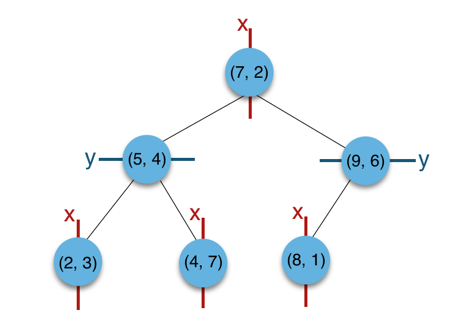
举例:给定一个二维空间的数据集 T={ (2,3),(5,4),(9,6),(4,7),(8,1),(7,2)}构建一个平衡kd树
a)构建根节点,选择x(1)轴,6个数据点在x维从小到大排序为(2,3),(4,7),(5,4),(7,2),(8,1),(9,6);其中值为(7,2)。(注:2,4,5,7,8,9在数学中的中值为(5 + 7)/2=6,但因该算法的中值需在点集合之内,所以本文中值计算用的是len(points)//2=3, points[3]=(7,2))
b)(2,3),(4,7),(5,4)挂在(7,2)节点的左子树,(8,1),(9,6)挂在(7,2)节点的右子树。
c)构建(7,2)节点的左子树时,点集合(2,3),(4,7),(5,4)此时的切分维度为y,中值为(5,4)作为分割平面,(2,3)挂在其左子树,(4,7)挂在其右子树。
d)构建(7,2)节点的右子树时,点集合(8,1),(9,6)此时的切分维度也为y,中值为(9,6)作为分割平面,(8,1)挂在其左子树。至此k-d tree构建完成。
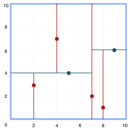
(kd)树特征空间划分:
5.2 最近邻搜索
用(kd)树的最近邻搜索
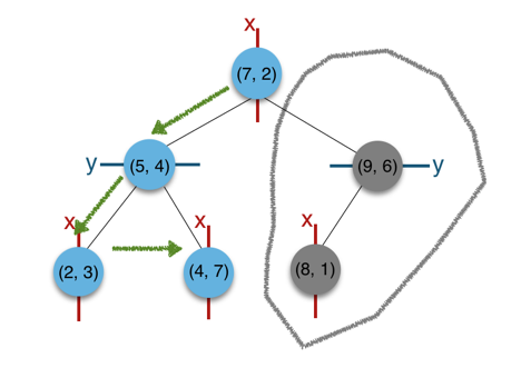
举例:给定点p,查询数据集中与其距离最近点的过程即为最近邻搜索。
如在上文构建好的k-d tree上搜索(3,5)的最近邻时,本文结合如下左右两图对二维空间的最近邻搜索过程作分析。
a)首先从根节点(7,2)出发,将当前最近邻设为(7,2),对该k-d tree作深度优先遍历。以(3,5)为圆心,其到(7,2)的距离为半径画圆(多维空间为超球面),可以看出(8,1)右侧的区域与该圆不相交,所以(8,1)的右子树全部忽略。
b)接着走到(7,2)左子树根节点(5,4),与原最近邻对比距离后,更新当前最近邻为(5,4)。以(3,5)为圆心,其到(5,4)的距离为半径画圆,发现(7,2)右侧的区域与该圆不相交,忽略该侧所有节点,这样(7,2)的整个右子树被标记为已忽略。
c)遍历完(5,4)的左右叶子节点,发现与当前最优距离相等,不更新最近邻。所以(3,5)的最近邻为(5,4)。

5.3 (kd)树代码实现
#kd-tree每个节点中主要包含的数据结构
class KdNode(object):
    def __init__(self, dom_elt, split, left, right):
        self.dom_elt = dom_elt  #k维向量节点(k维空间中的一个样本点)
        self.split = split  #整数(进行分割维度的序号)
        self.left = left  #该节点分割超平面左子空间构成的kd-tree
        self.right = right  #该节点分割超平面右子空间构成的kd-tree

class KdTree(object):
    def __init__(self, data):
        k = len(data[0])  #数据维度

        def CreateNode(split, data_set):  #按第split维划分数据集exset创建KdNode
            if not data_set:  #数据集为空
                return None

            data_set.sort(key=lambda x: x[split])
            split_pos = len(data_set)//2
            median = data_set[split_pos]  #中位数分割点
            split_next = (split+1)%k

            #递归创建kd-tree
            return KdNode(
                median,
                split,
                CreateNode(split_next, data_set[:split_pos]),  #创建左子树
                CreateNode(split_next, data_set[split_pos+1:])  #创建右子树
            )
        self.root = CreateNode(0, data)  # 从第0维分量开始构建kd树,返回根节点

#kd-tree的前序遍历
def preorder(root):
    print(root.dom_elt)
    if root.left:
        preorder(root.left)
    if root.right:
        preorder(root.right)


# 对构建好的kd树进行搜索,寻找与目标点最近的样本点
from math import sqrt
from collections import namedtuple

# 定义一个namedtuple,分别存放最近坐标点、最近距离和访问过的节点数
result = namedtuple("Result_tuple",
                    "nearest_point  nearest_dist  nodes_visited")

def find_nearest(tree, point):
    k = len(point)  #数据维度

    def travel(kd_node, target, max_dist):
        if kd_node is None:
            return result([0]*k, float("inf"), 0)  # python中用float("inf")和float("-inf")表示正负无穷
        nodes_visited = 1
        s = kd_node.split  #进行分割的维度
        pivot = kd_node.dom_elt  #进行分割的轴

        if target[s] <= pivot[s]:  # 如果目标点第s维小于分割轴的对应值(目标离左子树更近)
            near_node = kd_node.left  # 下一个访问节点为左子树根节点
            further_node = kd_node.right  #同时记录下右子树
        else:   #目标离右子树更近
            near_node = kd_node.right
            further_node = kd_node.left

        temp1 = travel(near_node, target, max_dist)  #遍历找到包含目标点的区域
        nearest = temp1.nearest_point  #以此叶结点作为“当前最近点”
        dist = temp1.nearest_dist  #更新最近距离

        nodes_visited += temp1.nodes_visited

        if dist < max_dist:
            max_dist = dist # 最近点将在以目标点为球心,max_dist为半径的超球体内
        temp_dist = abs(pivot[s] - target[s])  # 第s维上目标点与分割超平面的距离
        if max_dist < temp_dist:  #判断超球体是否与超平面相交
            return result(nearest, dist, nodes_visited)  #不相交则直接返回 不用继续判断

        #计算目标点与分割点的欧式距离
        temp_dist = sqrt(sum((p1-p2)**2 for p1, p2 in zip(pivot, target)))

        if temp_dist<dist: #如果更近
            nearest = pivot #更新最近点
            dist = temp_dist #更新最近距离
            max_dist = dist  #更新超球体半径

        #检查另一个子结点对应的区域是否有更近的点
        temp2 = travel(further_node, target, max_dist)

        nodes_visited += temp2.nodes_visited
        if temp2.nearest_dist < dist:  #如果另一个子节点内存在更近距离
            nearest = temp2.nearest_point  #更新最近点
            dist = temp2.nearest_dist  #更新最近距离
        return result(nearest, dist, nodes_visited)
    return travel(tree.root, point, float("inf"))  #从根节点开始递归

data = [[2,3],[5,4],[9,6],[4,7],[8,1],[7,2]]
kd = KdTree(data)
preorder(kd.root)
#输出
[7, 2]
[5, 4]
[2, 3]
[4, 7]
[9, 6]
[8, 1]

from time import clock
from random import random

#产生一个k维随机向量 每维分量值在0-1之间
def random_point(k):
    return [random() for _ in range(k)]

#产生n个k维随机向量
def random_pints(k, n):
    return [random_point(k) for _ in range(n)]

ret = find_nearest(kd, [3, 4.5])
print(ret)

#输出
Result_tuple(nearest_point=[2, 3], nearest_dist=1.8027756377319946, nodes_visited=4)

N = 400000
t0 = clock()
kd2 = KdTree(random_pints(3, N))  # 构建包含四十万个3维空间样本点的kd树
ret2 = find_nearest(kd2, [0.1, 0.5, 0.8])  # 四十万个样本点中寻找离目标最近的点
t1 = clock()

print ("time: ",t1-t0, "s")  #time:  6.427965869746692 s

print (ret2)
#输出
Result_tuple(nearest_point=[0.10636624893047031, 0.49814097780478606, 0.7967586569829902], nearest_dist=0.007381828602787445, nodes_visited=42)
6 KNN小结
KNN优点:精度高、对异常值不敏感、无数据输入假定。
KNN缺点:计算复杂度高、空间复杂度高。
参考:统计学习方法 机器学习实战 kd树算法原理及实现