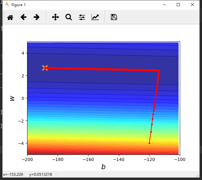
 1 import numpy as np
 2 import matplotlib.pyplot as plt
 3
 4 x_data = [338,333,328,207,226,25,179,60,208,606]
 5 y_data = [640,633,619,393,428,27,193,66,226,1591]
 6
 7
 8 #生成从-200到-100的数,不包括-100
 9 #x轴
10 x = np.arange(-200,-100,1)
11 #y轴
12 y = np.arange(-5,5,0.1)
13 #存储对应的误差
14 Z = np.zeros((len(x),len(y)))
15 #x横向平铺给X,y纵向平铺给Y
16 #X,Y = np.meshgrid(x,y)
17 for i in range(len(x)):
18     for j in range(len(y)):
19         b = x[i]
20         w = y[j]
21         #按行进行计算误差
22         Z[j][i] = 0
23         #误差和
24         for n in range(len(x_data)):
25             Z[j][i] = Z[j][i] + (y_data[n] - b - w*x_data[n])**2
26         #归一化
27         Z[j][i] = Z[j][i]/len(x_data)
28
29
30 #y = b + w * x
31 b = -120
32 w = -4
33 #lr = 0.0000001
34 lr = 0.000001#学习速率
35 # lr = 0.00001
36 iteration = 100000
37
38 #记录每次求得的b和w
39 b_history = [b]
40 w_history = [w]
41
42 for i in range(iteration):
43     b_grad = 0.0
44     w_grad = 0.0
45
46     for n in range(len(x_data)):
47         b_grad = b_grad - 2.0*(y_data[n] - b - w*x_data[n])*1.0
48         w_grad = w_grad - 2.0 * (y_data[n] - b - w * x_data[n]) * x_data[n]
49     b = b - lr * b_grad
50     w = w - lr * w_grad
51
52     b_history.append(b)
53     w_history.append(w)
54
55 #五十种颜色  透明度:0.8
56 plt.contourf(x, y, Z, 50, alpha=0.8, cmap=plt.get_cmap('jet'))
57 #画出最优解的位置
58 plt.plot([-188.4],[2.67],'x',ms=12,markeredgewidth=3,color='orange')
59 plt.plot(b_history,w_history,'o-',ms = 3,lw = 1.5,color = 'red')
60 #绘制坐标轴
61 plt.xlim(-200,-100)
62 plt.ylim(-5,5)
63 #给坐标轴命名
64 plt.xlabel(r'$b$',fontsize=16)
65 plt.ylabel(r'$w$',fontsize=16)
66 plt.show()
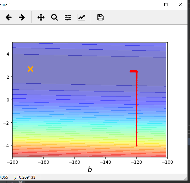
动态调整学习速率
 1 import numpy as np
 2 import matplotlib.pyplot as plt
 3
 4 x_data = [338,333,328,207,226,25,179,60,208,606]
 5 y_data = [640,633,619,393,428,27,193,66,226,1591]
 6
 7
 8 #生成从-200到-100的数,不包括-100
 9 #x轴
10 x = np.arange(-200,-100,1)
11 #y轴
12 y = np.arange(-5,5,0.1)
13 #存储对应的误差
14 Z = np.zeros((len(x),len(y)))
15 #x横向平铺给X,y纵向平铺给Y
16 #X,Y = np.meshgrid(x,y)
17 for i in range(len(x)):
18     for j in range(len(y)):
19         b = x[i]
20         w = y[j]
21         #按行进行计算误差
22         Z[j][i] = 0
23         #误差和
24         for n in range(len(x_data)):
25             Z[j][i] = Z[j][i] + (y_data[n] - b - w*x_data[n])**2
26         #归一化
27         Z[j][i] = Z[j][i]/len(x_data)
28
29
30 #y = b + w * x
31 b = -120
32 w = -4
33 #lr = 0.0000001
34 lr = 1#学习速率
35 # lr = 0.00001
36 iteration = 100000
37
38 #记录每次求得的b和w
39 b_history = [b]
40 w_history = [w]
41
42 lr_b = 0
43 lr_w = 0
44
45
46 for i in range(iteration):
47     b_grad = 0.0
48     w_grad = 0.0
49
50     for n in range(len(x_data)):
51         b_grad = b_grad - 2.0*(y_data[n] - b - w*x_data[n])*1.0
52         w_grad = w_grad - 2.0 * (y_data[n] - b - w * x_data[n]) * x_data[n]
53
54     lr_b = lr_b + b_grad ** 2
55     lr_w = lr_w + w_grad ** 2
56     # b = b - lr * b_grad
57     # w = w - lr * w_grad
58     #动态调整学习速率
59     b = b - lr/np.sqrt(lr_b) * b_grad
60     w = w - lr/np.sqrt(lr_w) * w_grad
61
62     b_history.append(b)
63     w_history.append(w)
64
65 #五十种颜色  透明度:0.8
66 plt.contourf(x, y, Z, 50, alpha=0.8, cmap=plt.get_cmap('jet'))
67 #画出最优解的位置
68 plt.plot([-188.4],[2.67],'x',ms=12,markeredgewidth=3,color='orange')
69 plt.plot(b_history,w_history,'o-',ms = 3,lw = 1.5,color = 'red')
70 #绘制坐标轴
71 plt.xlim(-200,-100)
72 plt.ylim(-5,5)
73 #给坐标轴命名
74 plt.xlabel(r'$b$',fontsize=16)
75 plt.ylabel(r'$w$',fontsize=16)
76 plt.show()