本章主要介绍几种可替代普通最小二乘拟合的其他一些方法。
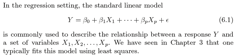
Why might we want to use another fitting procedure instead of least squares?
better prediction accuracy(预测精度) and better model interpretability(模型解释力).
主要介绍三种方法:
Subset Selection、Shrinkage、Dimension Reduction
6.1Subset Selection
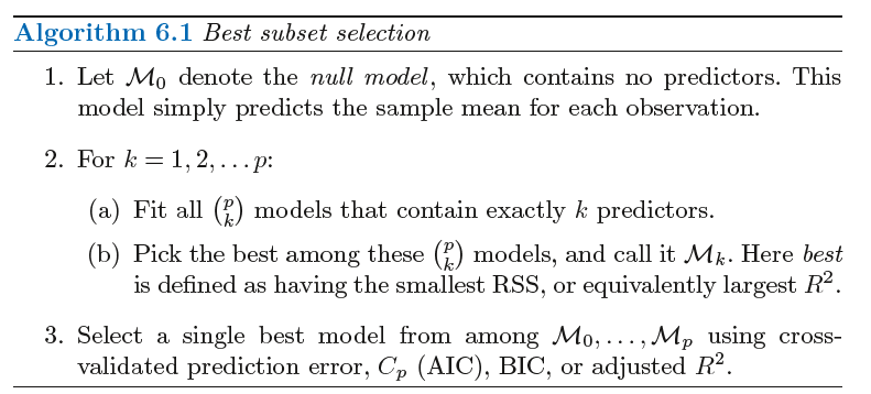
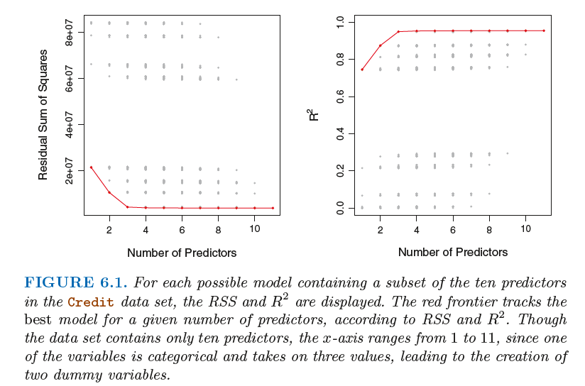
6.1.1 Best Subset Selection
该方法从p 个预测变量中挑选出与响应变最相关的变量形成子集,再对缩减的变量集合使用最小二乘方法。
6.1.2 Stepwise Selection
由于运算效率的限制,当p 很大时,最优子集选择方法不再适用,而且也存在一些统计学上的问题。随着搜索空间始增大,
通过此方法找到的模型虽然在训练数据上有较好的表现,但对新数据并不具备良好的预测能力。从一个巨大搜索空间中得到
的模型通常会有过拟合和系数估计方差高的问题。
跟最优子集选择相比,逐步选择的优点是限制了搜索空间,从而提高了运算效率。
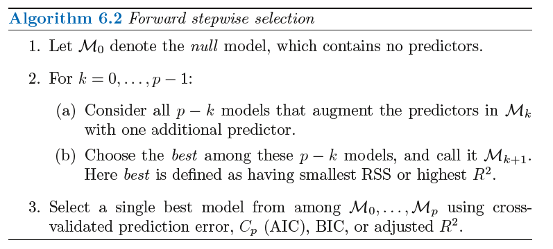
向前逐步选择
向后逐步选择

向后选择方法将满足样本量n 大于变放个数p (保证全模型可以被拟合)的条件。相反,
向前逐步选择即使在n <p 的情况下也可以使用,因此当p非常大的时候,向前逐步选择是唯
一可行的方法。
混合方法
还有一种将向前和向后逐步选择方法进行综合的方法。与向前逐步选择类似,该方法逐次将变量加人模型中,然而在加入新变量的同时,
该方法也移除不能提升模型拟合效果的变量。这种方法在试图达到最优子集选择效果的同时也保留了向前和向后逐步选择在计算效率上的优势。
6.1.3 Choosing the Optimal Model
In order to select the best model with respect to test error, we need to estimate this test error. There are two common approaches:
1. We can indirectly estimate test error by making an adjustment to the training error to account for the bias due to overfitting.
2. We can directly estimate the test error, using either a validation set approach or a cross-validation approach, as discussed in Chapter 5.
We consider both of these approaches below.
6.2 Shrinkage Methods
我们可以使用对系数进行约束或加罚的技巧对包含p个预测变量的模型进行拟合,也就是说,将系数估计值往零的方向压缩。
可以显著减少估计量方差。两种最常用的方法是岭回归(ridge regression) 和llasso。
6.2.1 Ridge Regression
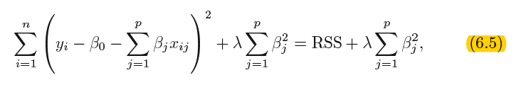
其中λ 是一个调节参数(turning parameter) ,将单独确定。
![]() called a shrinkage penalty is shrinkage small when β1, . . . , βp are close to zero, and so it has the effect of shrinking penalty the estimates of βj towards zero.
called a shrinkage penalty is shrinkage small when β1, . . . , βp are close to zero, and so it has the effect of shrinking penalty the estimates of βj towards zero.
Selecting a good value for λ is critical;we defer this discussion to Section 6.2.3, where we use cross-validation

It is best to apply ridge regression after standardizing the predictors, using the formula

Why Does Ridge Regression Improve Over Least Squares?
Ridge regression’s advantage over least squares is rooted in the bias-variance trade-off.
In particular, when the number of variables p is almost as large as the number of observations n, as in the example in Figure 6.5, the least
squares estimates will be extremely variable. And if p > n, then the least squares estimates do not even have a unique solution,whereas
ridge regression can still perform well by trading off a small increase in bias for a large decrease in variance. Hence, ridge regression works
best in situations where the least squares estimates have high variance.(当n<p或n=p时最小二乘法将有很大的方差,然而岭回归用一点偏差的增加大大地减小了方差的值)
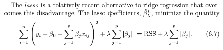
6.2.2 The Lasso
Ridge regression does have one obvious disadvantage. Unlike best subset, forward stepwise, and backward stepwise selection,
which will generally select models that involve just a subset of the variables, ridge regression will include all p predictors in the final
model.The penalty λβ2 j in (6.5) will shrink all of the coefficients towards zero, but it will not set any of them exactly to zero (unless λ = ∞).
This may not be a problem for prediction accuracy, but it can create a challenge in model interpretation in settings in which the number
of variables p is quite large. (岭回归不会将任何一个变量的系数压缩至0,这种设定不影响预测精度,但当变量个数非常大的时候,不便于模型解释)
For example, in the Credit data set, it appears that the most important variables are income, limit, rating, and student. So we might wish to
build a model including just these predictors. However, ridge regression will always generate a model involving all ten predictors. Increasing
the value of λ will tend to reduce the magnitudes of the coefficients, but will not result in exclusion of any of the variables.
写不下去了,看书吧。。。。
6.2.3 Selecting the Tuning Parameter
We then select the tuning parameter value for which the cross-validation error is smallest. Finally, the model is re-fit using all of
the available observations and the selected value of the tuning parameter.

6.3 Dimension Reduction Methods
We now explore a class of approaches that transform the predictors and then fit a least squares model using the transformed variables.
We will refer to these techniques as dimension reduction methods
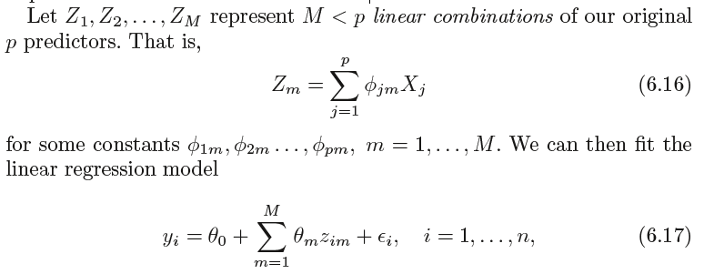
using least squares. Note that in (6.17), the regression coefficients are given
by θ0, θ1, . . . , θM. If the constants φ1m, φ2m, . . . , φpm are chosen wisely, then
such dimension reduction approaches can often outperform least squares
regression. In other words, fitting (6.17) using least squares can lead to
better results than fitting (6.1) using least squares.
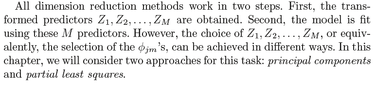
6.3.1Principal Components Regression(主成分回归)
Principal components analysis (PCA) is a popular approach for deriving principal components analysis
a low-dimensional set of features from a large set of variables.