科学计算与可视化
一,numpy库的安装与使用
1,numpy库的安装
用这个比较快 :pip3 install scipy -i https://pypi.tuna.tsinghua.edu.cn/simple
2,numpy库的使用
NumPy(Numerical Python) 是 Python 语言的一个扩展程序库,支持大量的维度数组与矩阵运算,此外也针对数组运算提供大量的数学函数库。
NumPy 是一个运行速度非常快的数学库,主要用于数组计算,包含:
(1) 一个强大的N维数组对象 ndarray
(2)广播功能函数
(3) 整合 C/C++/Fortran 代码的工具
(4)线性代数、傅里叶变换、随机数生成等功能
NumPy 通常与 SciPy(Scientific Python)和 Matplotlib(绘图库)一起使用, 这种组合广泛用于替代 MatLab,是一个强大的科学计算环境,有助于我们通过 Python 学习数据科学或者机器学习。
NumPy 数据类型
numpy 支持的数据类型比 Python 内置的类型要多很多,基本上可以和 C 语言的数据类型对应上,其中部分类型对应为 Python 内置的类型。下表列举了常用 NumPy 基本类型。
| 名称 | 描述 |
|---|---|
| bool_ | 布尔型数据类型(True 或者 False) |
| int_ | 默认的整数类型(类似于 C 语言中的 long,int32 或 int64) |
| intc | 与 C 的 int 类型一样,一般是 int32 或 int 64 |
| intp | 用于索引的整数类型(类似于 C 的 ssize_t,一般情况下仍然是 int32 或 int64) |
| int8 | 字节(-128 to 127) |
| int16 | 整数(-32768 to 32767) |
| int32 | 整数(-2147483648 to 2147483647) |
| int64 | 整数(-9223372036854775808 to 9223372036854775807) |
| uint8 | 无符号整数(0 to 255) |
| uint16 | 无符号整数(0 to 65535) |
| uint32 | 无符号整数(0 to 4294967295) |
| uint64 | 无符号整数(0 to 18446744073709551615) |
| float_ | float64 类型的简写 |
| float16 | 半精度浮点数,包括:1 个符号位,5 个指数位,10 个尾数位 |
| float32 | 单精度浮点数,包括:1 个符号位,8 个指数位,23 个尾数位 |
| float64 | 双精度浮点数,包括:1 个符号位,11 个指数位,52 个尾数位 |
| complex_ | complex128 类型的简写,即 128 位复数 |
| complex64 | 复数,表示双 32 位浮点数(实数部分和虚数部分) |
| complex128 | 复数,表示双 64 位浮点数(实数部分和虚数部分) |
实例1:
1 import numpy as np
2 # 使用标量类型
3 dt = np.dtype(np.int32)
4 print(dt)
结果:
1 int32
实例2:
1 import numpy as np
2 # int8, int16, int32, int64 四种数据类型可以使用字符串 'i1', 'i2','i4','i8' 代替
3 dt = np.dtype('i4')
4 print(dt)
结果
1 int32
实例3
1 import numpy as np
2 # 字节顺序标注
3 dt = np.dtype('<i4')
4 print(dt)
结果
1 int32
实例4
1 # 首先创建结构化数据类型
2 import numpy as np
3 dt = np.dtype([('age',np.int8)])
4 print(dt)
结果
[('age', 'i1')]
二,matplotlib的安装与使用
1,matplotlib的安装
python -m pip install matplotlib
2,matplotlib的使用
Matplotlib 可能是 Python 2D-绘图领域使用最广泛的套件。它能让使用者很轻松地将数据图形化,并且提供多样化的输出格式。这里将会探索 matplotlib 的常见用法。
来个例子更具体:
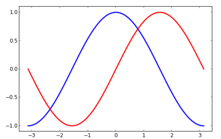
 1 # 导入 matplotlib 的所有内容(nympy 可以用 np 这个名字来使用)
 2 from pylab import *
 3
 4 # 创建一个 8 * 6 点(point)的图,并设置分辨率为 80
 5 figure(figsize=(8,6), dpi=80)
 6
 7 # 创建一个新的 1 * 1 的子图,接下来的图样绘制在其中的第 1 块(也是唯一的一块)
 8 subplot(1,1,1)
 9
10 X = np.linspace(-np.pi, np.pi, 256,endpoint=True)
11 C,S = np.cos(X), np.sin(X)
12
13 # 绘制余弦曲线,使用蓝色的、连续的、宽度为 1 (像素)的线条
14 plot(X, C, color="blue", linewidth=1.0, linestyle="-")
15
16 # 绘制正弦曲线,使用绿色的、连续的、宽度为 1 (像素)的线条
17 plot(X, S, color="green", linewidth=1.0, linestyle="-")
18
19 # 设置横轴的上下限
20 xlim(-4.0,4.0)
21
22 # 设置横轴记号
23 xticks(np.linspace(-4,4,9,endpoint=True))
24
25 # 设置纵轴的上下限
26 ylim(-1.0,1.0)
27
28 # 设置纵轴记号
29 yticks(np.linspace(-1,1,5,endpoint=True))
30
31 # 以分辨率 72 来保存图片
32 # savefig("exercice_2.png",dpi=72)
33
34 # 在屏幕上显示
35 show()

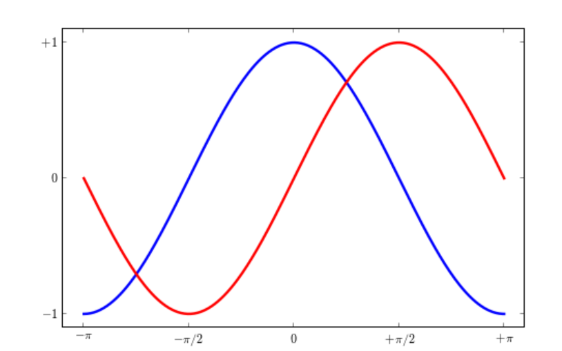
改变线条的颜色和粗细
1 ...
2 figure(figsize=(10,6), dpi=80)
3 plot(X, C, color="blue", linewidth=2.5, linestyle="-")
4 plot(X, S, color="red",  linewidth=2.5, linestyle="-")
5 ...

设置图片边界
1 xmin ,xmax = X.min(), X.max()
2 ymin, ymax = Y.min(), Y.max()
3
4 dx = (xmax - xmin) * 0.2
5 dy = (ymax - ymin) * 0.2
6
7 xlim(xmin - dx, xmax + dx)
8 ylim(ymin - dy, ymax + dy)
设置记号
1 ...
2 xticks([-np.pi, -np.pi/2, 0, np.pi/2, np.pi],
3        [r'$-pi$', r'$-pi/2$', r'$0$', r'$+pi/2$', r'$+pi$'])
4
5 yticks([-1, 0, +1],
6        [r'$-1$', r'$0$', r'$+1$'])
7 ...

 1 import numpy as np
 2 import matplotlib.pyplot as plt
 3
 4 # 中文和负号的正常显示
 5 plt.rcParams['font.sans-serif'] = 'Microsoft YaHei'
 6 plt.rcParams['axes.unicode_minus'] = False
 7
 8 # 绘图风格
 9 plt.style.use('seaborn-pastel')
10
11 # 构造数据
12 values = [50,100,100,100,110,70]
13 feature = ['第一周','第二周','第三周','第四周','第五周','第六周']
14
15 N = len(values)
16 # 设置角度
17 angles=np.linspace(0, 2*np.pi, N, endpoint=False)
18 # 封闭雷达图
19 values=np.concatenate((values,[values[0]]))
20 angles=np.concatenate((angles,[angles[0]]))
21
22 # 绘图
23 fig=plt.figure()
24 ax = fig.add_subplot(111, polar=True)
25 # 绘制折线图
26 ax.plot(angles, values, 'o-', linewidth=2, label = '学号2019310143003')
27 # 填充颜色
28 ax.fill(angles, values, alpha=0.55)
29
30 # 添加标签
31 ax.set_thetagrids(angles * 180/np.pi, feature)
32 # 设置雷达图的范围
33 ax.set_ylim(0,110)
34 # 添加标题
35 plt.title('tantan的成绩单')
36
37 # 添加网格线
38 ax.grid(True)
39 # 设置图例
40 plt.legend(loc = 'best')
41 # 显示图形
42 plt.show()
