SIFT特征提取与检索
SIFT特征提取
Harris函数可以很好的检测角点,这与角点本身的特性有关,这些角点在图像旋转的情况下也能被检测到,但是如果减小(或增加)图像的大小,可能会丢失图像的某些部分,或者有可能增加角点的质量。
这种特征损失现象需要用一种与图像比例无关的角点检测方法来解决——尺度不变特征变换(Scale-Invariant Feature Transform , SIFT),该函数会对不同的图像尺度(尺度不变特征变换)输出相同的结果。SIFT 会通过一个特征向量来描述关键点周围区域情况,而不检测关键点,其核心问题是将同一目标在不同时间、不同分辨率、不同光照、不同方向的情况下所成的像对应起来。
SIFT特征检测的步骤
- 尺度空间的极值检测:搜索所有尺度空间上的图像,通过高斯微分函数来识别潜在的对尺度和旋转不变的兴趣点。
- 特征点定位:在每个候选的位置上,通过一个拟合精细模型来确定位置尺度,关键点的选取依据他们的稳定程度。
- 特征方向赋值: 基于图像局部的梯度方向,分配给每个关键点位置一个或多个方向,后续的所有操作都是对于关键点的方向、尺度和位置进行变换,从而提供这些特征的不变性。
- 特征点描述: 在每个特征点周围的邻域内,在选定的尺度上测量图像的局部梯度,这些梯度被变换成一种表示,这种表示允许比较大的局部形状的变形和光照变换。
描述子
为了实现旋转不变性,基于每个点周围图像梯度的方向和大小,SIFT 描述子又引入了参考方向。SIFT 描述子使用主方向描述参考方向。主方向使用方向直方图(以大小为权重)来度量
检测兴趣点
使用开源工具包 VLFeat 提供的二进制文件来计算图像的 SIFT 特征
这里说明要安装VLFeat,否则是没法运行代码的,具体的安装方法我在网上找了一种:https://blog.csdn.net/weixin_44037639/article/details/88628253 描述的很详细,可以参照其进行安装,但是我下载vlfeat-0.9.21-bin.tar.gz 的安装包就无法解压,一直报错,所以我就下了9.20的。

需要注意的是括号后要有r 还有最后要有一个空格,否则还是无法运行代码的。
SIFT实验
构造出一个小的数据集
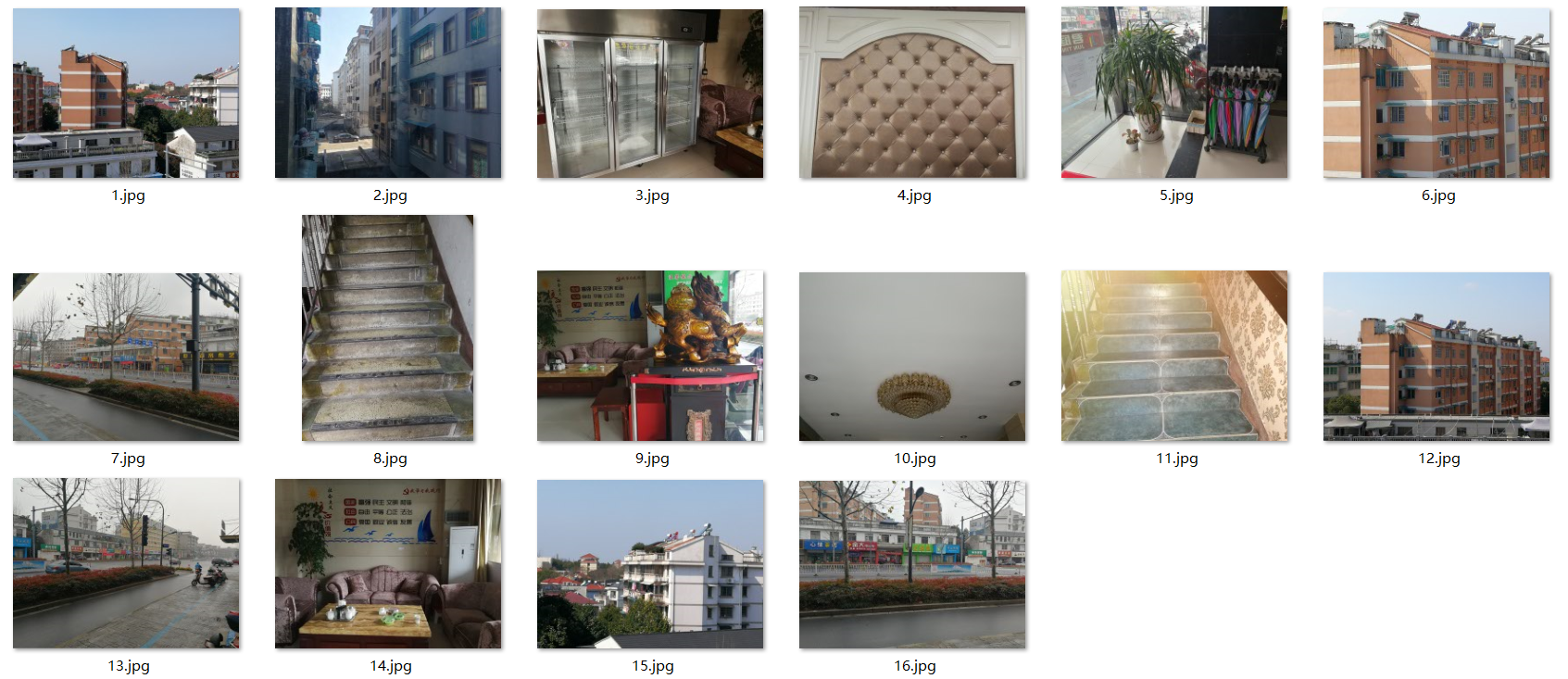
实现数据集中,每张图片的SIFT特征提取,并展示特征点
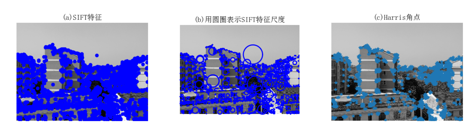
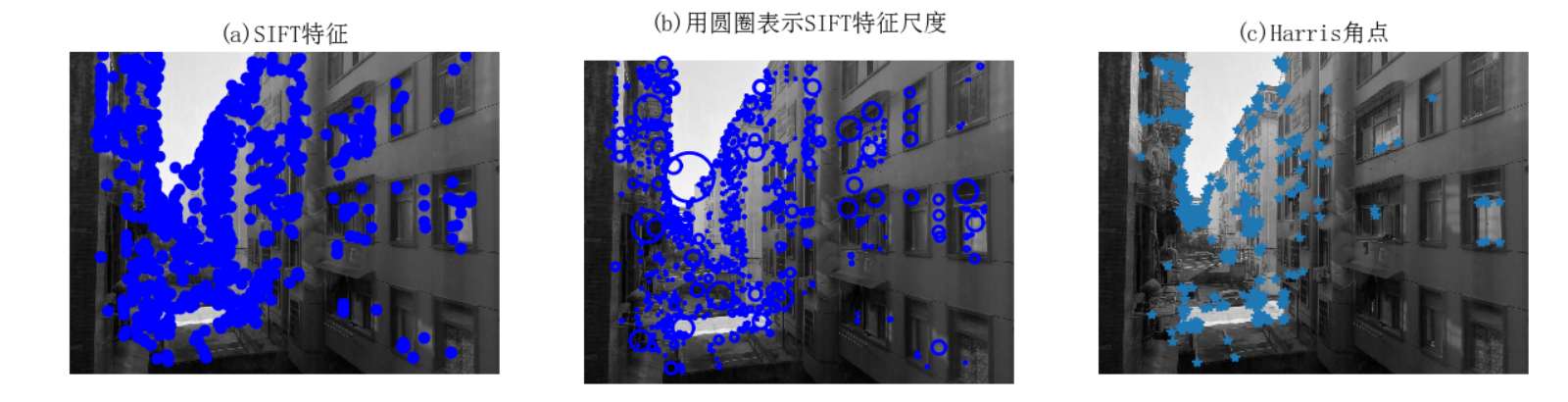

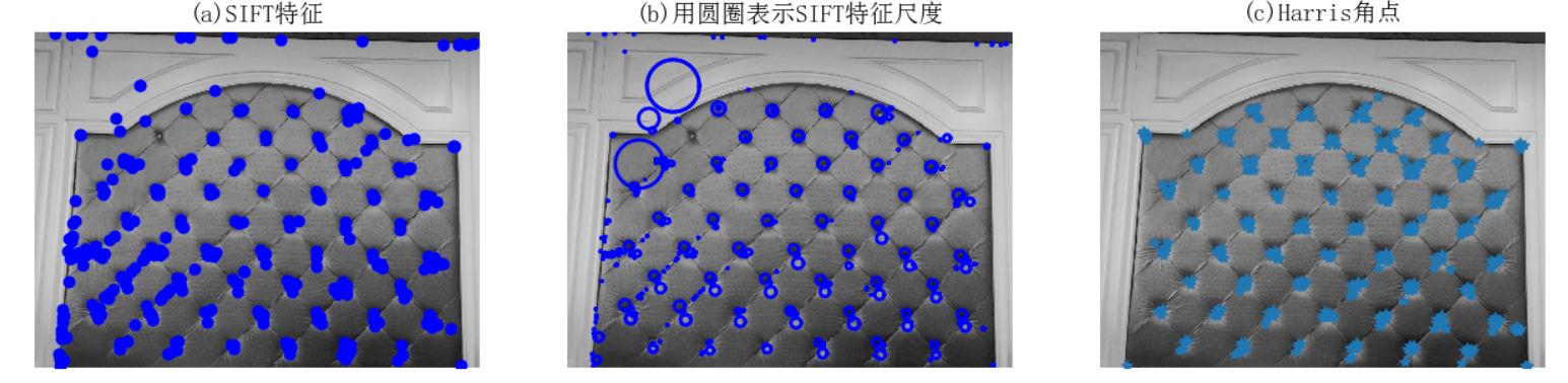

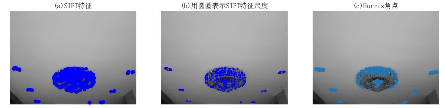
# -*- coding: utf-8 -*-
from PIL import Image
from pylab import *
from PCV.localdescriptors import sift
from PCV.localdescriptors import harris

# 添加中文字体支持
from matplotlib.font_manager import FontProperties

font = FontProperties(fname=r"c:windowsfontsSimSun.ttc", size=14)

imname = 'E:/迅雷下载/test_pic/2/10.jpg'
im = array(Image.open(imname).convert('L'))
sift.process_image(imname, 'empire.sift')
l1, d1 = sift.read_features_from_file('empire.sift')

figure()
gray()
subplot(131)
sift.plot_features(im, l1, circle=False)
title(u'(a)SIFT特征', fontproperties=font)
subplot(132)
sift.plot_features(im, l1, circle=True)
title(u'(b)用圆圈表示SIFT特征尺度', fontproperties=font)

# 检测harris角点
harrisim = harris.compute_harris_response(im)

subplot(133)
filtered_coords = harris.get_harris_points(harrisim, 6, 0.1)
imshow(im)
plot([p[1] for p in filtered_coords], [p[0] for p in filtered_coords], '*')
axis('off')
title(u'(c)Harris角点', fontproperties=font)

show()
SIFT特征检测算法与Harris 角点检测算法所选择特征点的位置不同,SIFT检测算法检测的精确度比后者更加好,它会对每个关键点周围的区域计算特征向量,因此它主要包括两个操作:检测和计算,操作的返回值是关键点信息和描述符,最后在图像上绘制关键点
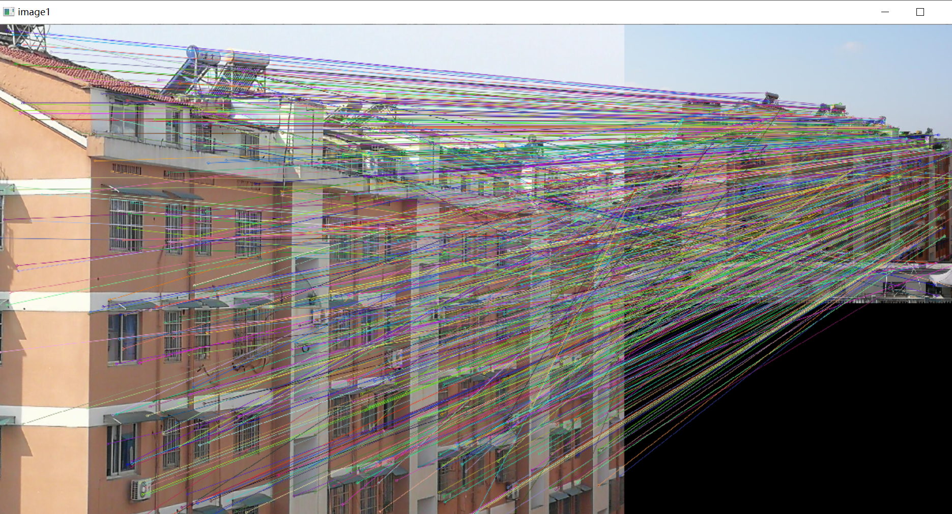
给定两张图片,计算其SIFT特征匹配结果
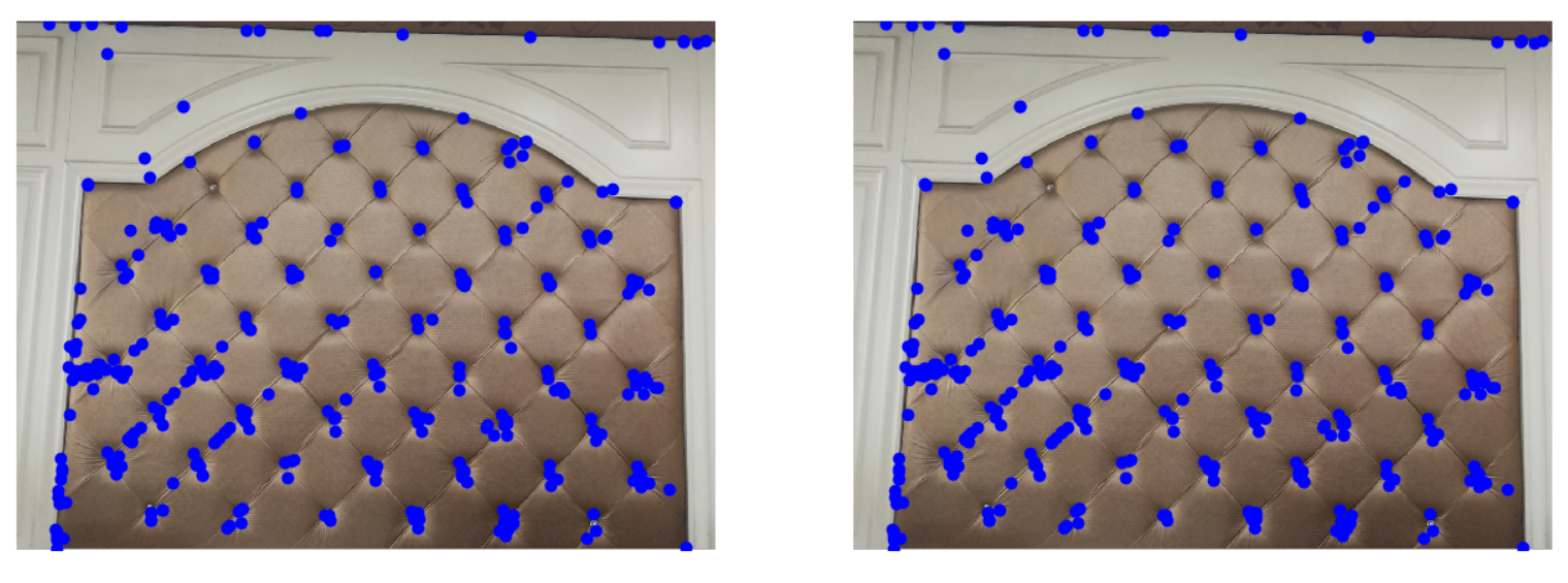

from PIL import Image
from pylab import *
import sys
from PCV.localdescriptors import sift

if len(sys.argv) >= 3:
    im1f, im2f = sys.argv[1], sys.argv[2]
else:
    im1f = 'E:/迅雷下载/test_pic/2/4.jpg'
    im2f = 'E:/迅雷下载/test_pic/2/4.jpg'
im1 = array(Image.open(im1f))
im2 = array(Image.open(im2f))

sift.process_image(im1f, 'out_sift_1.txt')
l1, d1 = sift.read_features_from_file('out_sift_1.txt')
figure()
gray()
subplot(121)
sift.plot_features(im1, l1, circle=False)

sift.process_image(im2f, 'out_sift_2.txt')
l2, d2 = sift.read_features_from_file('out_sift_2.txt')
subplot(122)
sift.plot_features(im2, l2, circle=False)

# matches = sift.match(d1, d2)
matches = sift.match_twosided(d1, d2)
print ('{} matches'.format(len(matches.nonzero()[0])) )
figure()
gray()
sift.plot_matches(im1, im2, l1, l2, matches, show_below=True)
show()
SIFT算法的实质是在不同的尺度空间上查找关键点(特征点),并计算出关键点的方向。SIFT所查找到的关键点是一些十分突出,不会因光照,仿射变换和噪音等因素而变化的点,如角点、边缘点、暗区的亮点及亮区的暗点等。但是对于光滑的平面貌似就没有特别好的效果,检测的效果没有Harris角点检测算法好。
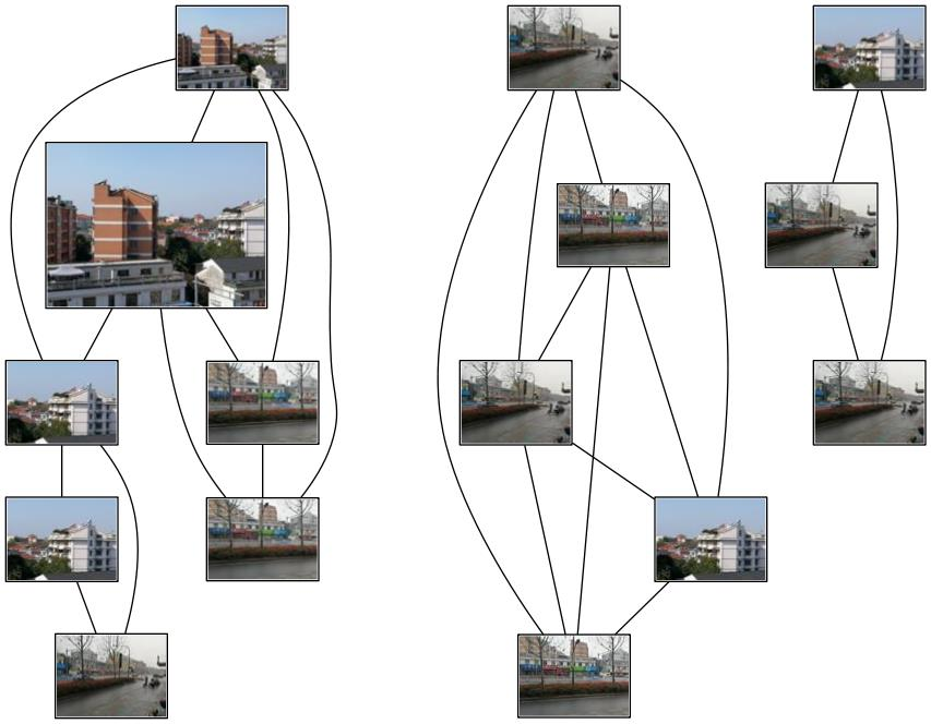
匹配地理标记
然后我重复运行了几次,每次结果都会有偏差,但是大体上还是没有太大出入


我采集的数据集中有一张比较特殊,麒麟这张图片的特征可能是特征点太多太杂,导致它跟房屋和马路都有一定的相似程度,可以考虑把这张照片剔除数据集....
我拍的照片组成的数据集有楼房有马路,本来应该是楼房跟楼房之间匹配程度高,马路跟马路之间匹配程度高,但是运行的结果显示楼房的图片跟马路的图片也有一定的相似程度,我觉得原因可能是因为马路的照片中背景包含了楼房,所以SIFT特征匹配检测到了楼房的特征,使得楼房的照片跟马路的照片有一定的相似程度。
可以看出,SIFT特征检测对于建筑物这些图有很强的实用性,能够将远处、近处、侧面、光照不同的相似图片的共同点匹配出来,即便是远处模糊的建筑物同样能检测出特征加以匹配。
同时,对于信息量很大的图片依旧能较为准确的找到特征,我拍摄的时候有些起雾,马路照片中的房屋较为模糊,SIFT特征匹配算法仍能将其特征与房屋图片匹配,就是运行代码的时候跑的时间有点久,运算的时间没有Harris角点检测算法快,但是精度更高是肯定的。
# -*- coding: utf-8 -*-
import json
import os
import urllib
# import urlparse
import urllib.request
from pylab import *
from PIL import Image
from PCV.localdescriptors import sift
from PCV.tools import imtools
import pydot

download_path = "E:/迅雷下载/test_pic/2"
path = "E:/迅雷下载/test_pic/2/"

imlist = imtools.get_imlist(download_path)
nbr_images = len(imlist)

featlist = [imname[:-3] + 'sift' for imname in imlist]
for i, imname in enumerate(imlist):
    sift.process_image(imname, featlist[i])

matchscores = zeros((nbr_images, nbr_images))

for i in range(nbr_images):
    for j in range(i, nbr_images):  # only compute upper triangle
        print('comparing ', imlist[i], imlist[j])
        l1, d1 = sift.read_features_from_file(featlist[i])
        l2, d2 = sift.read_features_from_file(featlist[j])
        matches = sift.match_twosided(d1, d2)
        nbr_matches = sum(matches > 0)
        print('number of matches = ', nbr_matches)
        matchscores[i, j] = nbr_matches

# copy values
for i in range(nbr_images):
    for j in range(i + 1, nbr_images):  # no need to copy diagonal
        matchscores[j, i] = matchscores[i, j]

# 可视化

threshold = 2  # min number of matches needed to create link

g = pydot.Dot(graph_type='graph')  # don't want the default directed graph

for i in range(nbr_images):
    for j in range(i + 1, nbr_images):
        if matchscores[i, j] > threshold:
            # first image in pair
            im = Image.open(imlist[i])
            im.thumbnail((200, 200))
            filename = path + str(i) + '.jpg'
            im.save(filename)  # need temporary files of the right size
            g.add_node(pydot.Node(str(i), fontcolor='transparent', shape='rectangle', image=filename))

            # second image in pair
            im = Image.open(imlist[j])
            im.thumbnail((200, 200))
            filename = path + str(j) + '.jpg'
            im.save(filename)  # need temporary files of the right size
            g.add_node(pydot.Node(str(j), fontcolor='transparent', shape='rectangle', image=filename))

            g.add_edge(pydot.Edge(str(i), str(j)))
g.write_jpg('E:/迅雷下载/test_pic/2/finally.jpg')
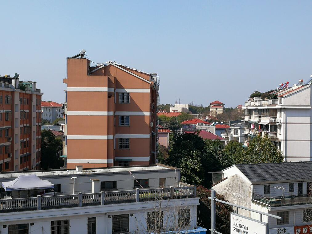
输入图片
输出图片
import os
import numpy as np
import matplotlib.image as mp
# from skimage import img_as_ubyte
from PIL import Image
from pylab import *
import sys
from PCV.localdescriptors import sift

# 添加中文字体支持
from matplotlib.font_manager import FontProperties
font = FontProperties(fname=r"c:windowsfontsSimSun.ttc", size=14)
path = "E:/迅雷下载/test_pic/2/"
filelist = os.listdir(path)  # 打开对应的文件夹
total_num = len(filelist)-1  #得到文件夹中图像的个数
matches_array=np.array([0,0,0,0,0,0,0,0,0,0,0,0,0,0,0])
result=np.array([0,0,0])
if len(sys.argv) >= 3:
    im1f, im2f = sys.argv[1], sys.argv[2]
else:
    im1f = 'E:/迅雷下载/test_pic/2/1.jpg'
im1 = array(Image.open(im1f))
sift.process_image(im1f, 'out_sift_1.txt')
l1, d1 = sift.read_features_from_file('out_sift_1.txt')
figure()
# subplot(2,2,1)
plt.axis('off')
title(u'原图',fontproperties=font)
imshow(Image.open(im1f))
for i in range(total_num):
    im2f = path + str(i + 1) + '.jpg' #拼接图像的读取地址
    im2 = array(Image.open(im2f))
    sift.process_image(im2f, 'out_sift_'+str(i+2)+'.txt')
    l2, d2 = sift.read_features_from_file('out_sift_'+str(i+2)+'.txt')
    matches = sift.match_twosided(d1, d2)
    matches_array[i] = len(matches.nonzero()[0])
print (matches_array)
for i in range(3):
    a = np.argmax(matches_array)
    im2f = path + str(a+1) + '.jpg' #拼接图像的读取地址
    subplot(1,3,i+1)
    plt.axis('off')
    mstr='matches:'+str(matches_array[a])
    # title(mstr,fontproperties=font)
    imshow(Image.open(im2f))
    matches_array[a]=0
show()
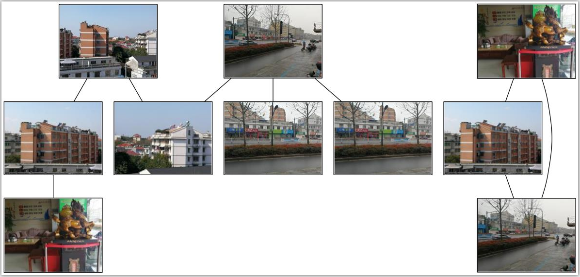
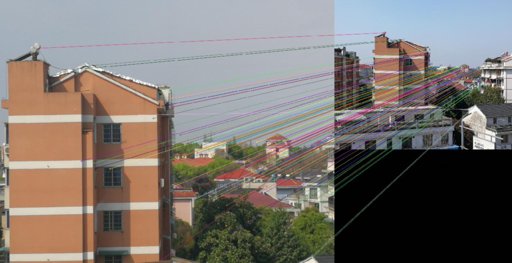
我拍摄了一账放大过的房屋图片,用它进行特征的匹配,在数据集中输出的图片是稍远出的这栋房屋还有另外一栋不同颜色的房屋,以及侧面的房屋图片,总体来说SIFT特征匹配相当精确,就是好像对颜色没啥感知,毕竟是根据房屋的特征来匹配,除了颜色,那两栋房屋的结构是相似的,匹配到一起很正常。
匹配精度不用说很好,但是运行速度真的不太给力,我已经尽量将图片压缩减小,但是运行时间还是要1-2分钟,耿别说再高清些的图片、数据集更大的集合,运行时间将会更久,不知道有啥能提高运行速度的方法。
无论是侧面还是类似的结构特征,SIFT算法都能精确的找出相似度高的图片,对于颜色、光照、雾天都能很好的应对。
RANSAC原理及算法应用
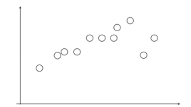
RANSAC是“RANdom SAmple Consensus”(随机一致性采样)的缩写,它于1981年由Fischler和Bolles最先提出。该方法是用来找到正确模型来拟合带有噪声数据的迭代方法。给定一个模型,例如点集之间 的单应性矩阵,RANSAC 基本的思想是,数据中包含正确的点和噪声点,合理的模型应该能够在描述正确数据点的同时摒弃噪声点。
RANSAC理论介绍
普通最小二乘是保守派:在现有数据下,如何实现最优。是从一个整体误差最小的角度去考虑,尽量谁也不得罪。
RANSAC是改革派:首先假设数据具有某种特性(目的),为了达到目的,适当割舍一些现有的数据。
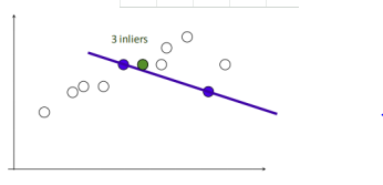
给出最小二乘拟合(红线)、RANSAC(绿线)对于一阶直线、二阶曲线的拟合对比:

可以看到RANSAC可以很好的拟合。RANSAC可以理解为一种采样的方式,所以对于多项式拟合、混合高斯模型(GMM)等理论上都是适用的。
RANSCA概述
RANSAC算法的输入是一组观测数据,一个可以解释或者适应于观测数据的参数化模型,一些可信的参数。
RANSAC通过反复选择数据中的一组随机子集来达成目标。被选取的子集被假设为局内点,并用下述方法进行验证:
1.有一个模型适应于假设的局内点,即所有的未知参数都能从假设的局内点计算得出。
2.用1中得到的模型去测试所有的其它数据,如果某个点适用于估计的模型,认为它也是局内点。
3.如果有足够多的点被归类为假设的局内点,那么估计的模型就足够合理。
4.然后,用所有假设的局内点去重新估计模型,因为它仅仅被初始的假设局内点估计过。
5.最后,通过估计局内点与模型的错误率来评估模型。
这个过程被重复执行固定的次数,每次产生的模型要么因为局内点太少而被舍弃,要么因为比现有的模型更好而被选用。
RANSAC的思路
随机选择四对匹配特征
根据DLT计算单应矩阵 H (唯一解)
对所有匹配点,计算映射误差ε= ||pi’, H pi||
根据误差阈值,确定inliers(例如3-5像素)
针对最大inliers集合,重新计算单应矩阵 H
1.在给定若干二维空间中的点,求直线 y=ax+b ,使得该直线对空间点的拟合误差最小。
2.随机选择两个点,根据这两个点构造直线,再计算剩余点到该直线的距离
给定阈值(距离小于设置的阈值的点为inliers),计算inliers数量
3.再随机选取两个点,同样计算inliers数量
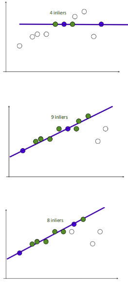
4.循环迭代,其中inliers最大的点集即为最大一致集,最后将该最大一致集里面的点利用最小二乘拟合出一条直线。
RANSAC模型测试

import numpy
import numpy as np
import scipy as sp
import scipy.linalg as sl

def ransac(data, model, n, k, t, d, debug = False, return_all = False):
    """
    参考:http://scipy.github.io/old-wiki/pages/Cookbook/RANSAC
    伪代码:http://en.wikipedia.org/w/index.php?title=RANSAC&oldid=116358182
    输入:
        data - 样本点
        model - 假设模型:事先自己确定
        n - 生成模型所需的最少样本点
        k - 最大迭代次数
        t - 阈值:作为判断点满足模型的条件
        d - 拟合较好时,需要的样本点最少的个数,当做阈值看待
    输出:
        bestfit - 最优拟合解(返回nil,如果未找到)

    iterations = 0
    bestfit = nil #后面更新
    besterr = something really large #后期更新besterr = thiserr
    while iterations < k
    {
        maybeinliers = 从样本中随机选取n个,不一定全是局内点,甚至全部为局外点
        maybemodel = n个maybeinliers 拟合出来的可能符合要求的模型
        alsoinliers = emptyset #满足误差要求的样本点,开始置空
        for (每一个不是maybeinliers的样本点)
        {
            if 满足maybemodel即error < t
                将点加入alsoinliers
        }
        if (alsoinliers样本点数目 > d)
        {
            %有了较好的模型,测试模型符合度
            bettermodel = 利用所有的maybeinliers 和 alsoinliers 重新生成更好的模型
            thiserr = 所有的maybeinliers 和 alsoinliers 样本点的误差度量
            if thiserr < besterr
            {
                bestfit = bettermodel
                besterr = thiserr
            }
        }
        iterations++
    }
    return bestfit
    """
    iterations = 0
    bestfit = None
    besterr = np.inf #设置默认值
    best_inlier_idxs = None
    while iterations < k:
        maybe_idxs, test_idxs = random_partition(n, data.shape[0])
        maybe_inliers = data[maybe_idxs, :] #获取size(maybe_idxs)行数据(Xi,Yi)
        test_points = data[test_idxs] #若干行(Xi,Yi)数据点
        maybemodel = model.fit(maybe_inliers) #拟合模型
        test_err = model.get_error(test_points, maybemodel) #计算误差:平方和最小
        also_idxs = test_idxs[test_err < t]
        also_inliers = data[also_idxs,:]
        if debug:
            print ('test_err.min()',test_err.min())
            print ('test_err.max()',test_err.max())
            print ('numpy.mean(test_err)',numpy.mean(test_err))
            print ('iteration %d:len(alsoinliers) = %d' %(iterations, len(also_inliers)) )
        if len(also_inliers > d):
            betterdata = np.concatenate( (maybe_inliers, also_inliers) ) #样本连接
            bettermodel = model.fit(betterdata)
            better_errs = model.get_error(betterdata, bettermodel)
            thiserr = np.mean(better_errs) #平均误差作为新的误差
            if thiserr < besterr:
                bestfit = bettermodel
                besterr = thiserr
                best_inlier_idxs = np.concatenate( (maybe_idxs, also_idxs) ) #更新局内点,将新点加入
        iterations += 1
        if bestfit is None:
            raise ValueError("did't meet fit acceptance criteria")
        if return_all:
            return bestfit,{'inliers':best_inlier_idxs}
        else:
            return bestfit


def random_partition(n, n_data):
    """return n random rows of data and the other len(data) - n rows"""
    all_idxs = np.arange(n_data) #获取n_data下标索引
    np.random.shuffle(all_idxs) #打乱下标索引
    idxs1 = all_idxs[:n]
    idxs2 = all_idxs[n:]
    return idxs1, idxs2

class LinearLeastSquareModel:
    #最小二乘求线性解,用于RANSAC的输入模型
    def __init__(self, input_columns, output_columns, debug = False):
        self.input_columns = input_columns
        self.output_columns = output_columns
        self.debug = debug

    def fit(self, data):
        A = np.vstack( [data[:,i] for i in self.input_columns] ).T #第一列Xi-->行Xi
        B = np.vstack( [data[:,i] for i in self.output_columns] ).T #第二列Yi-->行Yi
        x, resids, rank, s = sl.lstsq(A, B) #residues:残差和
        return x #返回最小平方和向量

    def get_error(self, data, model):
        A = np.vstack( [data[:,i] for i in self.input_columns] ).T #第一列Xi-->行Xi
        B = np.vstack( [data[:,i] for i in self.output_columns] ).T #第二列Yi-->行Yi
        B_fit = sp.dot(A, model) #计算的y值,B_fit = model.k*A + model.b
        err_per_point = np.sum( (B - B_fit) ** 2, axis = 1 ) #sum squared error per row
        return err_per_point

def test():
    #生成理想数据
    n_samples = 500 #样本个数
    n_inputs = 1 #输入变量个数
    n_outputs = 1 #输出变量个数
    A_exact = 20 * np.random.random((n_samples, n_inputs))#随机生成0-20之间的500个数据:行向量
    perfect_fit = 60 * np.random.normal( size = (n_inputs, n_outputs) ) #随机线性度即随机生成一个斜率
    B_exact = sp.dot(A_exact, perfect_fit) # y = x * k

    #加入高斯噪声,最小二乘能很好的处理
    A_noisy = A_exact + np.random.normal( size = A_exact.shape ) #500 * 1行向量,代表Xi
    B_noisy = B_exact + np.random.normal( size = B_exact.shape ) #500 * 1行向量,代表Yi

    if 1:
        #添加"局外点"
        n_outliers = 100
        all_idxs = np.arange( A_noisy.shape[0] ) #获取索引0-499
        np.random.shuffle(all_idxs) #将all_idxs打乱
        outlier_idxs = all_idxs[:n_outliers] #100个0-500的随机局外点
        A_noisy[outlier_idxs] = 20 * np.random.random( (n_outliers, n_inputs) ) #加入噪声和局外点的Xi
        B_noisy[outlier_idxs] = 50 * np.random.normal( size = (n_outliers, n_outputs)) #加入噪声和局外点的Yi
    #setup model
    all_data = np.hstack( (A_noisy, B_noisy) ) #形式([Xi,Yi]....) shape:(500,2)500行2列
    input_columns = range(n_inputs)  #数组的第一列x:0
    output_columns = [n_inputs + i for i in range(n_outputs)] #数组最后一列y:1
    debug = False
    model = LinearLeastSquareModel(input_columns, output_columns, debug = debug) #类的实例化:用最小二乘生成已知模型

    linear_fit,resids,rank,s = sp.linalg.lstsq(all_data[:,input_columns], all_data[:,output_columns])

    #run RANSAC 算法
    ransac_fit, ransac_data = ransac(all_data, model, 50, 1000, 7e3, 300, debug = debug, return_all = True)

    if 1:
        import pylab

        sort_idxs = np.argsort(A_exact[:,0])
        A_col0_sorted = A_exact[sort_idxs] #秩为2的数组

        if 1:
            pylab.plot( A_noisy[:,0], B_noisy[:,0], 'k.', label = 'data' ) #散点图
            pylab.plot( A_noisy[ransac_data['inliers'], 0], B_noisy[ransac_data['inliers'], 0], 'bx', label = "RANSAC data" )
        else:
            pylab.plot( A_noisy[non_outlier_idxs,0], B_noisy[non_outlier_idxs,0], 'k.', label='noisy data' )
            pylab.plot( A_noisy[outlier_idxs,0], B_noisy[outlier_idxs,0], 'r.', label='outlier data' )

        pylab.plot( A_col0_sorted[:,0],
                    np.dot(A_col0_sorted,ransac_fit)[:,0],
                    label='RANSAC fit' )
        pylab.plot( A_col0_sorted[:,0],
                    np.dot(A_col0_sorted,perfect_fit)[:,0],
                    label='exact system' )
        pylab.plot( A_col0_sorted[:,0],
                    np.dot(A_col0_sorted,linear_fit)[:,0],
                    label='linear fit' )
        pylab.legend()
        pylab.show()

if __name__ == "__main__":
    test()
测试景深丰富图片

sift特征提取匹配点

利用RANSAC算法剔除错误匹配点之后:
测试景深单一图片
sift特征提取匹配点
利用RANSAC算法剔除错误匹配点之后:

拍照的时候没注意,两张图片的大小没有统一,所以运行出来一张大一张小
很明显看出,RANSAC算法剔除错误匹配点之后,很多干扰点消失了,匹配的更加精准
即使是边缘的点也能精确的匹配到对应位置
还有就是两张图片的体积大小不同貌似不会对RANSAC算法造成太大的影响。
# -*- coding: utf-8 -*-
import cv2


import numpy as np

import random


def compute_fundamental(x1, x2):

    n = x1.shape[1]

    if x2.shape[1] != n:

        raise ValueError("Number of points don't match.")


    # build matrix for equations

    A = np.zeros((n, 9))

    for i in range(n):

        A[i] = [x1[0, i] * x2[0, i], x1[0, i] * x2[1, i], x1[0, i] * x2[2, i],

                x1[1, i] * x2[0, i], x1[1, i] * x2[1, i], x1[1, i] * x2[2, i],

                x1[2, i] * x2[0, i], x1[2, i] * x2[1, i], x1[2, i] * x2[2, i]]


    # compute linear least square solution

    U, S, V = np.linalg.svd(A)

    F = V[-1].reshape(3, 3)


    # constrain F

    # make rank 2 by zeroing out last singular value

    U, S, V = np.linalg.svd(F)

    S[2] = 0

    F = np.dot(U, np.dot(np.diag(S), V))


    return F / F[2, 2]


def compute_fundamental_normalized(x1, x2):

    """    Computes the fundamental matrix from corresponding points

        (x1,x2 3*n arrays) using the normalized 8 point algorithm. """


    n = x1.shape[1]

    if x2.shape[1] != n:

        raise ValueError("Number of points don't match.")


    # normalize image coordinates

    x1 = x1 / x1[2]

    mean_1 = np.mean(x1[:2], axis=1)

    S1 = np.sqrt(2) / np.std(x1[:2])

    T1 = np.array([[S1, 0, -S1 * mean_1[0]], [0, S1, -S1 * mean_1[1]], [0, 0, 1]])

    x1 = np.dot(T1, x1)


    x2 = x2 / x2[2]

    mean_2 = np.mean(x2[:2], axis=1)

    S2 = np.sqrt(2) / np.std(x2[:2])

    T2 = np.array([[S2, 0, -S2 * mean_2[0]], [0, S2, -S2 * mean_2[1]], [0, 0, 1]])

    x2 = np.dot(T2, x2)


    # compute F with the normalized coordinates

    F = compute_fundamental(x1, x2)

    # print (F)

    # reverse normalization

    F = np.dot(T1.T, np.dot(F, T2))


    return F / F[2, 2]


def randSeed(good, num = 8):

    '''

    :param good: 初始的匹配点对

    :param num: 选择随机选取的点对数量

    :return: 8个点对list

    '''

    eight_point = random.sample(good, num)

    return eight_point


def PointCoordinates(eight_points, keypoints1, keypoints2):

    '''

    :param eight_points: 随机八点

    :param keypoints1: 点坐标

    :param keypoints2: 点坐标

    :return:8个点

    '''

    x1 = []

    x2 = []

    tuple_dim = (1.,)

    for i in eight_points:

        tuple_x1 = keypoints1[i[0].queryIdx].pt + tuple_dim

        tuple_x2 = keypoints2[i[0].trainIdx].pt + tuple_dim

        x1.append(tuple_x1)

        x2.append(tuple_x2)

    return np.array(x1, dtype=float), np.array(x2, dtype=float)


def ransac(good, keypoints1, keypoints2, confidence,iter_num):

    Max_num = 0

    good_F = np.zeros([3,3])

    inlier_points = []

    for i in range(iter_num):

        eight_points = randSeed(good)

        x1,x2 = PointCoordinates(eight_points, keypoints1, keypoints2)

        F = compute_fundamental_normalized(x1.T, x2.T)

        num, ransac_good = inlier(F, good, keypoints1, keypoints2, confidence)

        if num > Max_num:

            Max_num = num

            good_F = F

            inlier_points = ransac_good

    print(Max_num, good_F)

    return Max_num, good_F, inlier_points


def computeReprojError(x1, x2, F):

    """

    计算投影误差

    """

    ww = 1.0/(F[2,0]*x1[0]+F[2,1]*x1[1]+F[2,2])

    dx = (F[0,0]*x1[0]+F[0,1]*x1[1]+F[0,2])*ww - x2[0]

    dy = (F[1,0]*x1[0]+F[1,1]*x1[1]+F[1,2])*ww - x2[1]

    return dx*dx + dy*dy


def inlier(F,good, keypoints1,keypoints2,confidence):

    num = 0

    ransac_good = []

    x1, x2 = PointCoordinates(good, keypoints1, keypoints2)

    for i in range(len(x2)):

        line = F.dot(x1[i].T)

        #在对极几何中极线表达式为[A B C],Ax+By+C=0,  方向向量可以表示为[-B,A]

        line_v = np.array([-line[1], line[0]])

        err = h = np.linalg.norm(np.cross(x2[i,:2], line_v)/np.linalg.norm(line_v))

        # err = computeReprojError(x1[i], x2[i], F)

        if abs(err) < confidence:

            ransac_good.append(good[i])

            num += 1

    return num, ransac_good


if __name__ =='__main__':


    im1 = 'E:/迅雷下载/test_pic/test1.jpg'
    im2 = 'E:/迅雷下载/test_pic/test2.jpg'


    print(cv2.__version__)

    psd_img_1 = cv2.imread(im1, cv2.IMREAD_COLOR)

    psd_img_2 = cv2.imread(im2, cv2.IMREAD_COLOR)

    # 3) SIFT特征计算

    sift = cv2.xfeatures2d.SIFT_create()

    # find the keypoints and descriptors with SIFT

    kp1, des1 = sift.detectAndCompute(psd_img_1, None)

    kp2, des2 = sift.detectAndCompute(psd_img_2, None)


    # FLANN 参数设计

    match = cv2.BFMatcher()

    matches = match.knnMatch(des1, des2, k=2)


    # Apply ratio test

    # 比值测试,首先获取与 A距离最近的点 B (最近)和 C (次近),

    # 只有当 B/C 小于阀值时(0.75)才被认为是匹配,

    # 因为假设匹配是一一对应的,真正的匹配的理想距离为0

    good = []

    for m, n in matches:

        if m.distance < 0.75 * n.distance:

            good.append([m])

    print(good[0][0])


    print("number of feature points:",len(kp1), len(kp2))

    print(type(kp1[good[0][0].queryIdx].pt))

    print("good match num:{} good match points:".format(len(good)))

    for i in good:

        print(i[0].queryIdx, i[0].trainIdx)


    Max_num, good_F, inlier_points = ransac(good, kp1, kp2, confidence=30, iter_num=500)

    # cv2.drawMatchesKnn expects list of lists as matches.

    # img3 = np.ndarray([2, 2])

    # img3 = cv2.drawMatchesKnn(img1, kp1, img2, kp2, good[:10], img3, flags=2)


    # cv2.drawMatchesKnn expects list of lists as matches.


    img3 = cv2.drawMatchesKnn(psd_img_1,kp1,psd_img_2,kp2,good,None,flags=2)

    img4 = cv2.drawMatchesKnn(psd_img_1,kp1,psd_img_2,kp2,inlier_points,None,flags=2)

    cv2.namedWindow('image1', cv2.WINDOW_NORMAL)

    cv2.namedWindow('image2', cv2.WINDOW_NORMAL)

    cv2.imshow("image1",img3)

    cv2.imshow("image2",img4)

    cv2.waitKey(0)#等待按键按下

    cv2.destroyAllWindows()#清除所有窗口
总结
- 匹配地理标记的测试中,运行结果经常发生波动,有几次甚至发生了图片缺失,但是大体上匹配的结果是正确的,不清楚为什么每次运行都会重新排列,明明上一次运行的相似度值都还在,可能是内存释放了所以又重新运行一遍。运行的结果图片是100*100的缩放图片,但是我感觉不太清晰,想要放大一些,调成了200*200的,运行出来还是100*100,而且更糊了....可能是我窗口大小调错了吧。
- 匹配中如果出现了特殊的照片,也就是特征点特别多的,很有可能会造成与多种类型的图片都有较高的相似度,我个人觉得就直接把这种图片剔除数据集吧。SIFT算法可能也不知道它该跟谁匹配。
- SIFT特征优点:尺度不变性 旋转不变性 光照不变性 鉴别性强,可识别的信息量丰富
- SIFT特征的缺点: 对于边缘光滑的目标无法准确提取特征点
- ransac是通过一堆点,对其中的一部分进行随机取样,用随机取得点拟合一条直线,再看这一堆点中满足这条直线方程的点占多少比例,如果这个比例大于某个阈值,则最终以所取模型表征这一堆点的模型。
- ransac能从包含大量局外点的数据集中估计出高精度的参数,也就是能匹配出更高相似度的点,进而去剔除噪点
- ransac对于景深丰富的图片有很好的匹配能力,能进一步加强SIFT算法的精确度