CCS

Matched Filter

The matched filter provides an alternative to the signal correlator for demodulating
the received signal r(t). A filter that is matched to the signal waveform s(t), where
0 <= t <= Tb, has an impulse response,

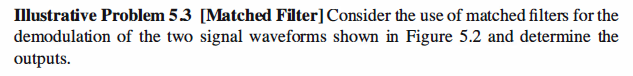
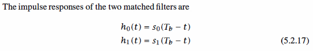
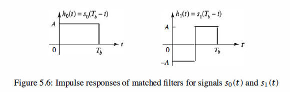
　　Note, Si(Tb - t) equals to the actions of folding Si(t) to get Si(-t) then delay it Tb( to the right, since Tb > 0) to obtain Si(Tb - t) .

Matlab Coding

 1 % MATLAB script
 2 
 3 % Initialization:
 4 K=20;       % Number of samples
 5 A=1;        % Signal amplitude
 6 l=0:K;

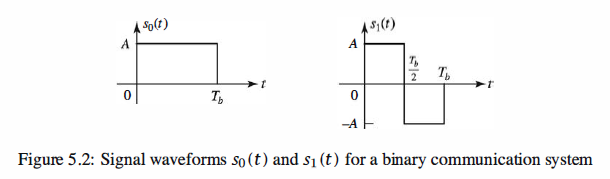
 7 % Defining signal waveforms:
 8 s_0=A*ones(1,K);
 9 s_1=[A*ones(1,K/2) -A*ones(1,K/2)];

10 % Initializing output signals:
11 y_0=zeros(1,K);
12 y_1=zeros(1,K);
13 
14 % Case 1: noise~N(0,0)
15 noise=random('Normal',0,0,1,K);
16     % Sub-case s = s_0:
17     s=s_0;
18     y=s+noise;  % received signal
19     y_0=conv(y,wrev(s_0));              % Matched Filter
20     y_1=conv(y,wrev(s_1));              % Matched Filter

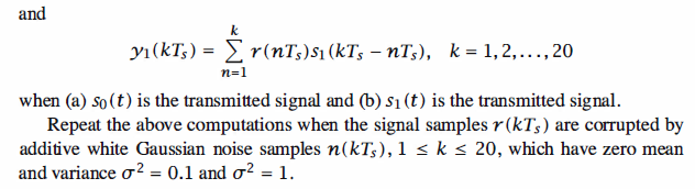
21     % Plotting the results:
22     subplot(3,2,1)
23     plot(l,[0 y_0(1:K)],'-k',l,[0 y_1(1:K)],'--k')
24     set(gca,'XTickLabel',{'0','5Tb','10Tb','15Tb','20Tb'})
25     axis([0 20 -30 30])
26     xlabel('(a) sigma^2= 0 & S_{0} is transmitted','fontsize',10)
27     % Sub-case s = s_1:
28     s=s_1;
29     y=s+noise;  % received signal
30     y_0=conv(y,wrev(s_0));
31     y_1=conv(y,wrev(s_1));
32     % Plotting the results:
33     subplot(3,2,2)
34     plot(l,[0 y_0(1:K)],'-k',l,[0 y_1(1:K)],'--k')
35     set(gca,'XTickLabel',{'0','5Tb','10Tb','15Tb','20Tb'})
36     axis([0 20 -30 30])
37     xlabel('(b) sigma^2= 0 & S_{1} is transmitted','fontsize',10)

38 % Case 2: noise~N(0,0.1)
39     noise=random('Normal',0,0.1,1,K);
40     % Sub-case s = s_0:
41     s=s_0;
42     y=s+noise;  % received signal
43     y_0=conv(y,wrev(s_0));
44     y_1=conv(y,wrev(s_1));
45     % Plotting the results:
46     subplot(3,2,3)
47     plot(l,[0 y_0(1:K)],'-k',l,[0 y_1(1:K)],'--k')
48     set(gca,'XTickLabel',{'0','5Tb','10Tb','15Tb','20Tb'})
49     axis([0 20 -30 30])
50     xlabel('(c) sigma^2= 0.1 & S_{0} is transmitted','fontsize',10)
51     % Sub-case s = s_1:
52     s=s_1;
53     y=s+noise;  % received signal
54     y_0=conv(y,wrev(s_0));
55     y_1=conv(y,wrev(s_1));
56     % Plotting the results:
57     subplot(3,2,4)
58     plot(l,[0 y_0(1:K)],'-k',l,[0 y_1(1:K)],'--k')
59     set(gca,'XTickLabel',{'0','5Tb','10Tb','15Tb','20Tb'})
60     axis([0 20 -30 30])
61     xlabel('(d) sigma^2= 0.1 & S_{1} is transmitted','fontsize',10)

62 % Case 3: noise~N(0,1)
63     noise=random('Normal',0,1,1,K);
64     % Sub-case s = s_0:
65     s=s_0;
66     y=s+noise;  % received signal
67     y_0=conv(y,wrev(s_0));
68     y_1=conv(y,wrev(s_1));
69     % Plotting the results:
70     subplot(3,2,5)
71     plot(l,[0 y_0(1:K)],'-k',l,[0 y_1(1:K)],'--k')
72     set(gca,'XTickLabel',{'0','5Tb','10Tb','15Tb','20Tb'})
73     axis([0 20 -30 30])
74     xlabel('(e) sigma^2= 1 & S_{0} is transmitted','fontsize',10)
75     % Sub-case s = s_1:
76     s=s_1;
77     y=s+noise;  % received signal
78     y_0=conv(y,wrev(s_0));
79     y_1=conv(y,wrev(s_1));
80     % Plotting the results:
81     subplot(3,2,6)
82     plot(l,[0 y_0(1:K)],'-k',l,[0 y_1(1:K)],'--k')
83     set(gca,'XTickLabel',{'0','5Tb','10Tb','15Tb','20Tb'})
84     axis([0 20 -30 30])
85     xlabel('(f) sigma^2= 1 & S_{1} is transmitted','fontsize',10)


Simulation Result

Reference,

　　1. <<Contemporary Communication System using MATLAB>> - John G. Proakis