CCS

Optimum Receiver for the AWGN Channel

The optimum receiver for the AWGN channel consists of two building blocks.

One is either a signal correlator or a matched filter . The other is a detector.

Signal Correlator

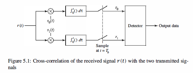
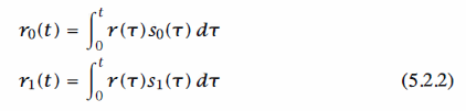
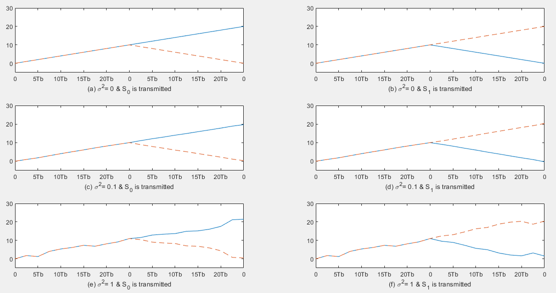
The signal correlator cross-correlates the received signal r ( t) with the two possible
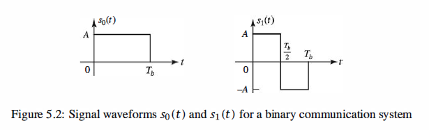
transmitted signals s0 ( t) and s1( t), as illustrated in Figure 5 .1. That is, the signal
correlator computes the two outputs,

in the interval 0 <= t <= Tb, samples the two outputs at t = Tb, and feeds the sampled

outputs to the detector.

Suppose that

Matlab coding

 1 % MATLAB script
 2 
 3 % Initialization:
 4 K=20;       % Number of samples
 5 A=1;        % Signal amplitude
 6 l=0:K;

 7 % Defining signal waveforms:
 8 s_0=A*ones(1,K);
 9 s_1=[A*ones(1,K/2) -A*ones(1,K/2)];

10 % Initializing output signals:
11 r_0=zeros(1,K);
12 r_1=zeros(1,K);
13 
14 % Case 1: noise~N(0,0)     sigma^2= 0
15 noise=random('Normal',0,0,1,K);
16     % Sub-case s = s_0:
17     s=s_0;
18     r=s+noise;  % received signal
19     for n=1:K
20         r_0(n)=sum(r(1:n).*s_0(1:n));    % Signal Correlator 
21         r_1(n)=sum(r(1:n).*s_1(1:n));
22     end
23     % Plotting the results:
24     subplot(3,2,1)
25     plot(l,[0 r_0],'-',l,[0 r_1],'--')
26     set(gca,'XTickLabel',{'0','5Tb','10Tb','15Tb','20Tb'})
27     axis([0 20 -5 30])
28     xlabel('(a) sigma^2= 0 & S_{0} is transmitted','fontsize',10)
29     % Sub-case s = s_1:
30     s=s_1;
31     r=s+noise;  % received signal
32     for n=1:K
33         r_0(n)=sum(r(1:n).*s_0(1:n));
34         r_1(n)=sum(r(1:n).*s_1(1:n));
35     end
36     % Plotting the results:
37     subplot(3,2,2)
38     plot(l,[0 r_0],'-',l,[0 r_1],'--')
39     set(gca,'XTickLabel',{'0','5Tb','10Tb','15Tb','20Tb'})
40     axis([0 20 -5 30])
41     xlabel('(b) sigma^2= 0 & S_{1} is transmitted','fontsize',10)

42 % Case 2: noise~N(0,0.1)      sigma^2= 0.1
43     noise=random('Normal',0,0.1,1,K);
44     % Sub-case s = s_0:
45     s=s_0;
46     r=s+noise;  % received signal
47     for n=1:K
48         r_0(n)=sum(r(1:n).*s_0(1:n));
49         r_1(n)=sum(r(1:n).*s_1(1:n));
50     end
51     % Plotting the results:
52     subplot(3,2,3)
53     plot(l,[0 r_0],'-',l,[0 r_1],'--')
54     set(gca,'XTickLabel',{'0','5Tb','10Tb','15Tb','20Tb'})
55     axis([0 20 -5 30])
56     xlabel('(c) sigma^2= 0.1 & S_{0} is transmitted','fontsize',10)
57     % Sub-case s = s_1:
58     s=s_1;
59     r=s+noise;  % received signal
60     for n=1:K
61         r_0(n)=sum(r(1:n).*s_0(1:n));
62         r_1(n)=sum(r(1:n).*s_1(1:n));
63     end
64     % Plotting the results:
65     subplot(3,2,4)
66     plot(l,[0 r_0],'-',l,[0 r_1],'--')
67     set(gca,'XTickLabel',{'0','5Tb','10Tb','15Tb','20Tb'})
68     axis([0 20 -5 30])
69     xlabel('(d) sigma^2= 0.1 & S_{1} is transmitted','fontsize',10)

70 % Case 3: noise~N(0,1)    sigma^2= 1
71     noise=random('Normal',0,1,1,K);
72     % Sub-case s = s_0:
73     s=s_0;
74     r=s+noise;  % received signal
75     for n=1:K
76         r_0(n)=sum(r(1:n).*s_0(1:n));          
77         r_1(n)=sum(r(1:n).*s_1(1:n));
78     end
79     % Plotting the results:
80     subplot(3,2,5)
81     plot(l,[0 r_0],'-',l,[0 r_1],'--')
82     set(gca,'XTickLabel',{'0','5Tb','10Tb','15Tb','20Tb'})
83     axis([0 20 -5 30])
84     xlabel('(e) sigma^2= 1 & S_{0} is transmitted','fontsize',10)
85     % Sub-case s = s_1:
86     s=s_1;
87     r=s+noise;  % received signal
88     for n=1:K
89         r_0(n)=sum(r(1:n).*s_0(1:n));
90         r_1(n)=sum(r(1:n).*s_1(1:n));
91     end
92     % Plotting the results:
93     subplot(3,2,6)
94     plot(l,[0 r_0],'-',l,[0 r_1],'--')
95     set(gca,'XTickLabel',{'0','5Tb','10Tb','15Tb','20Tb'})
96     axis([0 20 -5 30])
97     xlabel('(f) sigma^2= 1 & S_{1} is transmitted','fontsize',10)


Simulation Results

Reference,

　　1. <<Contemporary Communication System using MATLAB>> - John G. Proakis