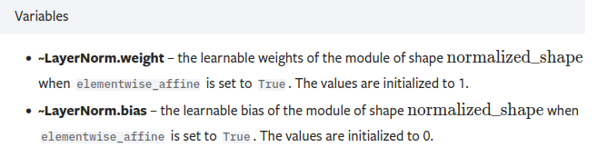
Layer Normalization
总览
- 针对同一通道数的图片的H*W进行层正则化,后面的γ和β是可以学习的参数,其中这两个的维度和最后一个的维度相同
- 例如特征图矩阵维度为[3, 577, 768], 那么γ和β的维度均为Tensor(768,)

step1:代码示例1
import torch
import torch.nn as nn


input = torch.tensor(
    [
    [
        [
            [2., 2.],
            [3., 3.]
        ],
        [
            [3., 3.],
            [2., 2.]
        ]
    ],
    [
        [
            [2., 2.],
            [3., 3.]
        ],
        [
            [3., 3.],
            [2., 2.]
        ]
    ]
]
)

print(input)
print(input.shape)  # torch.Size([2, 2, 2, 2])

layer_norm = nn.LayerNorm([2, 2, 2, 2], elementwise_affine=True)
output = layer_norm(input)

print(output)
"""
tensor([[[[-1.0000, -1.0000],
          [ 1.0000,  1.0000]],

         [[ 1.0000,  1.0000],
          [-1.0000, -1.0000]]],


        [[[-1.0000, -1.0000],
          [ 1.0000,  1.0000]],

         [[ 1.0000,  1.0000],
          [-1.0000, -1.0000]]]], grad_fn=<NativeLayerNormBackward>)
"""
# 总结
"""
根据公式
E(x) = ((2+2+3+3)*4)/16 = 2.5
Var(x) = {(2-2.5)**2 * 8 + (3-2.5)**2 * 8} / 16 = 0.5**2
带入公式可以得到:
y = (x - E(x)) / (var(x)**0.5)
可以得到output
"""
step2更改输入观察输出
import torch
import torch.nn as nn


input = torch.tensor(
    [
    [
        [
            [3., 2.],  # 这里将2 变成 3进行观察输出
            [3., 3.]
        ],
        [
            [3., 3.],
            [2., 2.]
        ]
    ],
    [
        [
            [2., 2.],
            [3., 3.]
        ],
        [
            [3., 3.],
            [2., 2.]
        ]
    ]
]
)

print(input)
print(input.shape)  # torch.Size([2, 2, 2, 2])

layer_norm = nn.LayerNorm([2, 2, 2, 2], elementwise_affine=True)
output = layer_norm(input)

print(output)
"""
tensor([[[[ 0.8819, -1.1339],
          [ 0.8819,  0.8819]],

         [[ 0.8819,  0.8819],
          [-1.1339, -1.1339]]],


        [[[-1.1339, -1.1339],
          [ 0.8819,  0.8819]],

         [[ 0.8819,  0.8819],
          [-1.1339, -1.1339]]]], grad_fn=<NativeLayerNormBackward>)
"""
# 总结
"""
由上述的公式可得,输入变化,整个输出都进行了改变
"""
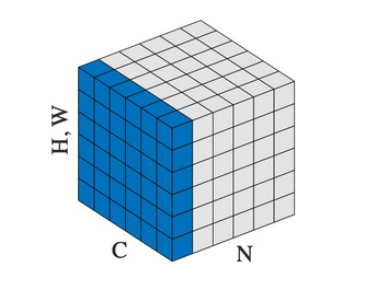
Batch Normalization
- 计算公式同上, 这里他的可学习参数与in_channel同
step1:代码示例1:
import torch
import torch.nn as nn


# With Learnable Parameters
m = nn.BatchNorm2d(2)

input = torch.tensor(
    [
    [
        [
            [2., 2.],
            [3., 3.]
        ],
        [
            [3., 3.],
            [2., 2.]
        ]
    ],
    [
        [
            [2., 2.],
            [3., 3.]
        ],
        [
            [3., 3.],
            [2., 2.]
        ]
    ]
]
)
print(input)
print(input.shape)  # torch.Size([2, 2, 2, 2])

output = m(input)
print(output)
"""
tensor([[[[-1.0000, -1.0000],
          [ 1.0000,  1.0000]],

         [[ 1.0000,  1.0000],
          [-1.0000, -1.0000]]],


        [[[-1.0000, -1.0000],
          [ 1.0000,  1.0000]],

         [[ 1.0000,  1.0000],
          [-1.0000, -1.0000]]]], grad_fn=<NativeBatchNormBackward>)
"""
# 总结:
"""
计算的是某个批次的正则
根据公式 以第一个批次为例:
E(x) = {2+2+3+3+2+2+3+3}/8 = 2.5
Var(x) = {(2-2.5)**2 * 4 + (3-2.5)**2 * 4}/8 = 0.5**2
带入公式可以得到:
y = (x - E(x)) / (var(x)**0.5)
可以得到output
"""
进行微小更改观察变化
import torch
import torch.nn as nn


# With Learnable Parameters
m = nn.BatchNorm2d(2)

input = torch.tensor(
    [
    [
        [
            [3., 2.],  # 这里2变成3来观察变化
            [3., 3.]
        ],
        [
            [3., 3.],
            [2., 2.]
        ]
    ],
    [
        [
            [2., 2.],
            [3., 3.]
        ],
        [
            [3., 3.],
            [2., 2.]
        ]
    ]
]
)
print(input)
print(input.shape)  # torch.Size([2, 2, 2, 2])

output = m(input)
print(output)
"""
tensor([[[[ 0.7746, -1.2910],
          [ 0.7746,  0.7746]],

         [[ 1.0000,  1.0000],
          [-1.0000, -1.0000]]],


        [[[-1.2910, -1.2910],
          [ 0.7746,  0.7746]],

         [[ 1.0000,  1.0000],
          [-1.0000, -1.0000]]]], grad_fn=<NativeBatchNormBackward>)
"""
# 总结:
"""
进行微小更改观察到,发生变化的是他同一批次里面的
"""
参考
layer_norm
batch_norm