Andrew Ng 的 Machine Learning 课程学习 (week2) Linear Regression

这学期一直在跟进 Coursera上的 Machina Learning 公开课, 老师Andrew Ng是coursera的创始人之一，Machine Learning方面的大牛。这门课程对想要了解和初步掌握机器学习的人来说是不二的选择。这门课程涵盖了机器学习的一些基本概念和方法，同时这门课程的编程作业对于掌握这些概念和方法起到了巨大的作用。

课程地址 https://www.coursera.org/learn/machine-learning

笔记主要是简要记录下课程内容,以及MATLAB编程作业....

Regression

回归,属于有监督学习中的一种方法。该方法的核心思想是从离散的统计数据中得到数学模型,然后将该数学模型用于预测或者分类。该方法处理的数据可以是多维的。课程最初介绍了一个房屋价格的基本问题,然后引出了线性回归的解决方法,然后针对误差问题做了概率解释。

与 Classification 的区别

   　　Regression: to predict the continuous valued output.

   　　Classification: to predict the discrete valued output.

Costfuntion

求最小值，局部最优或者全局最优

 

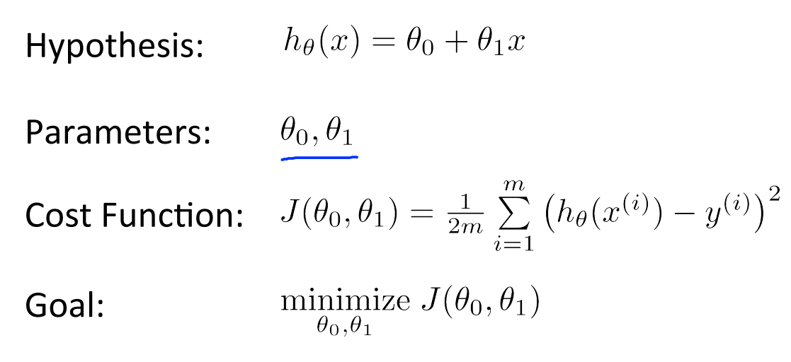
Grdient Descent

在选定线性回归模型后,只需要确定参数 θ,就可以将模型用来预测。然而 θ 需要在 J(θ)最小的情况下才能确定。因此问题归结为求极小值问题,使用梯度下降法。梯度下降法最大的问题是求得有可能是全局极小值,这与初始点的选取有关。

梯度下降法是按下面的流程进行的:

1)首先对 θ 赋值,这个值可以是随机的,也可以让 θ 是一个全零的向量。

2)改变 θ 的值,使得 J(θ)按梯度下降的方向进行减少。

梯度方向由 J(θ)对 θ 的偏导数确定,由于求的是极小值,因此梯度方向是偏导数的反方向。结果为

 

对于本章（week2)的编程作业题如下：

Week2 任务: Linear Regression

computeCost.m

function J = computeCost(X, y, theta)

% Initialize some useful values
m = length(y); % number of training examples

% You need to return the following variables correctly 
J = 0;

% ====================== YOUR CODE HERE ======================
% Instructions: Compute the cost of a particular choice of theta
%               You should set J to the cost.

h = X * theta;
E = h - y;
J = 1 / (2*m) * E' * E;
    
% ============================================================
end

gradientDescent.m

function [theta, J_history] = gradientDescent(X, y, theta, alpha, num_iters)

% Initialize some useful values
m = length(y); % number of training examples
J_history = zeros(num_iters, 1);
for iter = 1:num_iters

    % ====================== YOUR CODE HERE ======================
    % Instructions: Perform a single gradient step on the parameter vector
    %               theta. 
    %
    % Hint: While debugging, it can be useful to print out the values
    %       of the cost function (computeCost) and gradient here.
    %
    h = X * theta;
    E = h - y;
    theta = theta - alpha / m * X' * E;

    % =========================================================

    % Save the cost J in every iteration    
    J_history(iter) = computeCost(X, y, theta);
end
end

computeCostMulti.m

h = X * theta;
E = h - y;
J = 1 / (2*m) * E' * E;

gradientDescentMulti.m

h = X * theta;
E = h - y;
theta = theta - alpha / m * X' * E;