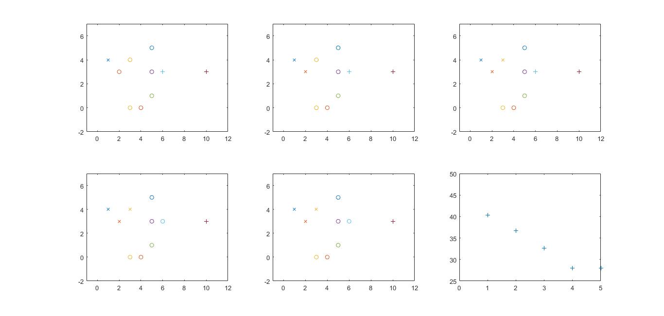
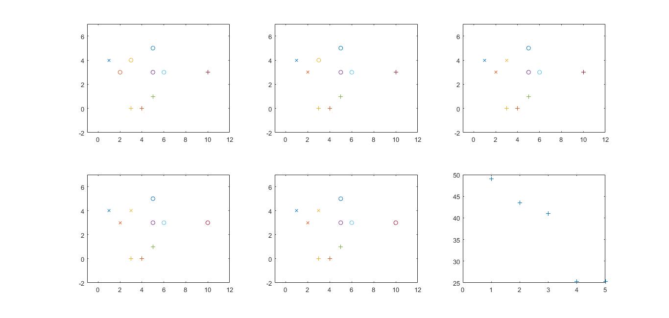
对散点进行二分聚类:
初始聚类中心的选择会影响分类次数甚至是否能成功分类, 算法采用离样本中心很近的两点作为初始聚类点.
程序如下:
% 设定分类次数,以自动调整分类精确度
% part1 得到散点数据并人工指定两个初始聚类中心点
clear all;clc;close all;  %注意,3c前面不能写东西,会被擦除.
x = [ [1,4]; [2,3]; [3,4]; [5,3]; [5,1]; [6,3]; [10,3]; [5,5 ] ];
cluster_count = 4;  % 聚类次数
len = size(x, 1);

intpx = 0;
intpy = 0;
for i = 1:len
    intpx = intpx + x(i, 1);
    intpy = intpy + x(i, 2);
end
intpx = intpx/len;
intpy = intpy/len;

% 注意坐标和矩阵要用方括号而不是圆括号
theta1 = [intpx + 0.01, intpy + 0.01];
theta2 = [intpx - 0.01, intpy - 0.01];

figure;
% part2 循环过程,其中,计数矩阵和索引矩阵的每次初始化都在循环中完成
for j = 1:cluster_count
    %    初始化索引和计数矩阵
    c = zeros(2, 1);
    %    画聚类中心点, 中点, 求斜率画中垂线
    subplot(2,2,j);
    title(['di',num2str(j)]);
    plot(theta1(1), theta1(2), '*'); hold on;
    plot(theta2(1), theta2(2), '*'); hold on;
    mid1 = (theta1(1) + theta2(1))/2;
    mid2 = (theta1(2) + theta2(2))/2;
    plot(mid1, mid2, '+'); hold on;
    axis([-2 10 -2 10])
    slope = (-1) * (theta1(1) - theta2(1))/(theta1(2) - theta2(2));
    t = 0:0.01:10;
    line = slope*(t-mid1) + mid2;
    plot(t, line); hold on;
    %    判断分类结果, 画出ox区分, 并得到新的双theta
    %    a 分类
    thetanew1 = [0, 0]; thetanew2 = [0, 0];
    for i = 1:len
        if (x(i,1)-theta1(1))^2 + (x(i,2)-theta1(2))^2 < (x(i,1)-theta2(1))^2 + (x(i,2)-theta2(2))^2
            y(i) = 1;
            c(1) = c(1) + 1;
            plot(x(i,1), x(i,2), 'x');hold on;
            thetanew1(1) = thetanew1(1) + x(i,1);
            thetanew1(2) = thetanew1(2) + x(i,2);
        else
            y(i) = 0;
            c(2) = c(2) + 1;
            plot(x(i,1), x(i, 2), 'o');hold on;
            thetanew2(1) = thetanew2(1) + x(i,1);
            thetanew2(2) = thetanew2(2) + x(i,2);
        end
    end
    theta1 = thetanew1/c(1);
    theta2 = thetanew2/c(2);
    %    b 双theta

    axis([-2 10 -2 10])
end

% 若第一次分类为初始值分类,则可见第三次分类已达最佳
输出图像如下:
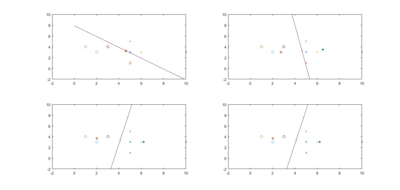
三分聚类:
% 三分聚类
% 2c
clc; close all;
% clear all is not really necesssary, beccause every variable with the same
% name
% 导入要分类的散点数据
x = [ [1,4]; [2,3]; [3,4]; [5,3]; [5,1]; [6,3]; [10,3]; [5,5 ]; [4, 0]; [3, 0] ];
%x = [ [1, 1]; [2, 1]; [2,2]; [8,1]; [8,2]; [8,3]; [4, 8]; [5, 8] ];
cluster_times = 4;
len = size(x, 1);
xxall = 0; xyall = 0;
for i = 1:len
    xxall = xxall + x(i, 1);
    xyall = xyall + x(i, 2);
end

xysum = [xxall, xyall];

intpx = 0;
intpy = 0;
for i = 1:len
    intpx = intpx + x(i, 1);
    intpy = intpy + x(i, 2);
end
intpx = intpx/len;
intpy = intpy/len;

% 注意坐标和矩阵要用方括号而不是圆括号
%{
theta1 = [intpx, intpy + 1.01];
theta2 = [intpx - 1.02, intpy + 1.03];
theta3 = [intpx + 1.04, intpy - 1.05];
%}

theta1 = x(1,:);
theta2 = x(2,:);
theta3 = x(10,:);

% 判断
for j = 1:cluster_times
    %    初始化索引和计数矩阵
    c = zeros(3, 1);
    %    画聚类中心点, 中点, 求斜率画中垂线
    %subplot(3,3,j);
    figure;
    % title(['di',num2str(j)]);

    % plot(mid1, mid2, '+'); hold on;
    axis([-2 10 -2 10])


    %    判断分类结果, 画出ox区分, 并得到新的双theta
    %    a 分类
    thetanew1 = [0, 0]; thetanew2 = [0, 0]; thetanew3 = [0, 0];
    for i = 1:len
        if (x(i,1)-theta1(1))^2 + (x(i,2)-theta1(2))^2 < (x(i,1)-theta2(1))^2 + (x(i,2)-theta2(2))^2 ...
                && ((x(i,1)-theta1(1))^2 + (x(i,2)-theta1(2))^2 < (x(i,1)-theta3(1))^2 + (x(i,2)-theta3(2))^2)
            y(i) = 0;
            c(1) = c(1) + 1;
            plot(x(i,1), x(i,2), 'x');hold on;
            thetanew1(1) = thetanew1(1) + x(i,1);
            thetanew1(2) = thetanew1(2) + x(i,2);
        elseif (x(i,1)-theta2(1))^2 + (x(i,2)-theta2(2))^2 < (x(i,1)-theta1(1))^2 + (x(i,2)-theta1(2))^2 ...
                && ((x(i,1)-theta2(1))^2 + (x(i,2)-theta2(2))^2 < (x(i,1)-theta3(1))^2 + (x(i,2)-theta3(2))^2)
            y(i) = 1;
            c(2) = c(2) + 1;
            plot(x(i,1), x(i, 2), 'o'); hold on;
            thetanew2(1) = thetanew2(1) + x(i,1);
            thetanew2(2) = thetanew2(2) + x(i,2);
        else
            y(i) = 2;
            c(3) = c(3) + 1;
            plot(x(i, 1), x(i, 2), '+'); hold on;
            thetanew3(1) = thetanew3(1) + x(i, 1);
            thetanew3(2) = thetanew3(2) + x(i, 2);
        end
    end
    theta1 = thetanew1/c(1);
    theta2 = thetanew2/c(2);
    theta3 = thetanew3/c(3);

    mid12 = (theta1 + theta2)/2;
    mid23 = (theta2 + theta3)/2;
    mid31 = (theta3 + theta1)/2;
    slope12 = (-1) * (theta1(1) - theta2(1))/(theta1(2) - theta2(2));  %负倒数通过交换分子分母得到
    slope23 = (-1) * (theta2(1) - theta3(1))/(theta2(2) - theta3(2));
    slope31 = (-1) * (theta3(1) - theta1(1))/(theta3(2) - theta1(2));

    t = 0:0.01:10;
    %t = 4.2:0.01:10;
    line12 = slope12*(t-mid12(1)) + mid12(2);
    plot(t, line12); hold on;

    %t = 0:0.01:4.2;
    line23 = slope23*(t-mid23(1)) + mid23(2);
    plot(t, line23); hold on;

    %t = 4.2:0.01:10;
    line31 = slope31*(t-mid31(1)) + mid31(2);
    plot(t, line31); hold on;
    %plot(theta1(1), theta1(2), '*');
    %plot(theta2(1), theta2(2), '*');
    %plot(theta3(1), theta3(2), '*');
    % 运行结果不能达到预期时先不要否定算法而是先检查一下细节
    %    b 双theta

    axis([-2 10 -2 10])
end
输出如下:
初始点theta1, theta2, theta3 选x1, x2, x10:
初始点选x1, x2, x7 就会陷入局部最优: