本文中,我们将使用前面已经实现的水波渗透算法来测定对于固定大小的网格,在不同开放概率p下发生渗透的概率。关于该部分的具体说明如下:
How many trials are needed to make a prediction on whether a grid generated with probability p percolates?
How many different values of p should be considered to determine the percolation probability q?
需要做多少次实验才能确定一个按概率p产生的网格是否渗透?
需要考虑多少个不同的p值才能确定渗透概率q?
For p=1, the grid will always percolate (there are no blocked locations) and for p=0 the grid will never percolate (all locations are blocked). Intuitively, for values of p close to 1, one expects that the majority of the trials will report percolation and for values of p close to 0 one expects very few percolations.
如果p=1,网络总是渗透(没有阻塞位置),如果p=0,网格不能渗透(所有位置都是阻塞的)。直观来讲,接近1的p值,我们会认为大多数的实验结果是渗透的,而接近0的p值,极少是渗透的。
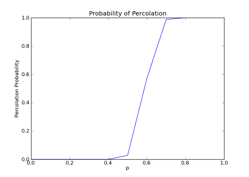
The goal is to generate a plot whose x-coordinate represents values of p (from 0 to 1) and whose y-coordinate represents q (also from 0 to 1). From the shape of the plot, you will make a prediction of the percolation probability.
目的是产生一个图,它的x座标表示p的值(从0到1),y座标表示q(也是从0到1)。从图的形状来看,你会对渗透作出一个预测。
Every point in the plot is obtained by running a number of trials. For a certain probability p, assume we are making t trials and s of the t randomly generated grids allow percolation. We set q = s/t and (p,q) is a point in the plot. It would be helpful if there were a formula allowing us to plot this function. However, such a formula does not exist.
图中的每个点是根据多次实验得出的。对于某一概率p,假设我们进行t次实验,t个随机产生的网格有s个允许渗透。我们设q=s/t,(p,q)是图中的一个点。如果存在一个准则允许我们图出这个函数,这对我们将很有帮助。然而,这样的准则并不存在。
Experimentally determine the percolation probability for a grid of size n=25. Remember that you need to decide how many values of p to consider and how many experiments to run for each value of p (you should set this quantity t to at leats 10). Plot the graph using Matplotlib or VPython. Place all code generating the plot into a file experiment_n_fixed.py (this file needs to import all files and libraries you use). In addition to the graph, discuss how you decided on the number of trials used and the probabilities p considered. State the observed percolation probability.
实验确定一个n=25的网格的渗透率。记住,你需要决定考虑p值的大小及对于每个p值,实验运行的次数(你应该设置t的大小至少为10)。使用Matplotlib或Vpython画图。把产生图的所有代码放到experiment_n_fixed.py文件(这一文件需要调用你需要用到的所有文件和库)下。除图之外,讨论一下你是怎样确定实验次数和考虑的概率p。说明观察到的渗透率。
那么这个实验的关键点就是在于p值的实验次数和每个p值的实验运行次数。
测试脚本如下:
from pylab import *
step = 0.01
trial_count = 100
size = 25
if __name__ == '__main__':
p = 0
results = []
while p < 1:
print 'Running for p =', p, '...'
perc_count = 0
for k in range(trial_count):
g = random_grid(size, p)
flow,perc = percolation_wave(g,trace=False)
if perc:
perc_count += 1
prob = float(perc_count)/trial_count
print 'percolation q=:',prob
results.append(prob)
p += step
print len(results)
#b = bar(arange(0,1,step), results, width=step, color='r')
plot(arange(0,1,step), results)
xlabel('p')
ylabel('Percolation Probability')
title('Probability of Percolation')
show()
根据概率论的原理,样本空间越大,那么得到的值与实际结果相比越精确。不过考虑到运行时间的情况,我们不可能选择非常大的试验次数。
我对p值的(例如设P增幅为0.01,那么N=1/0.01=100)总执行步数N和每个p值的实验运行次数M进行了尝试,结果如下:
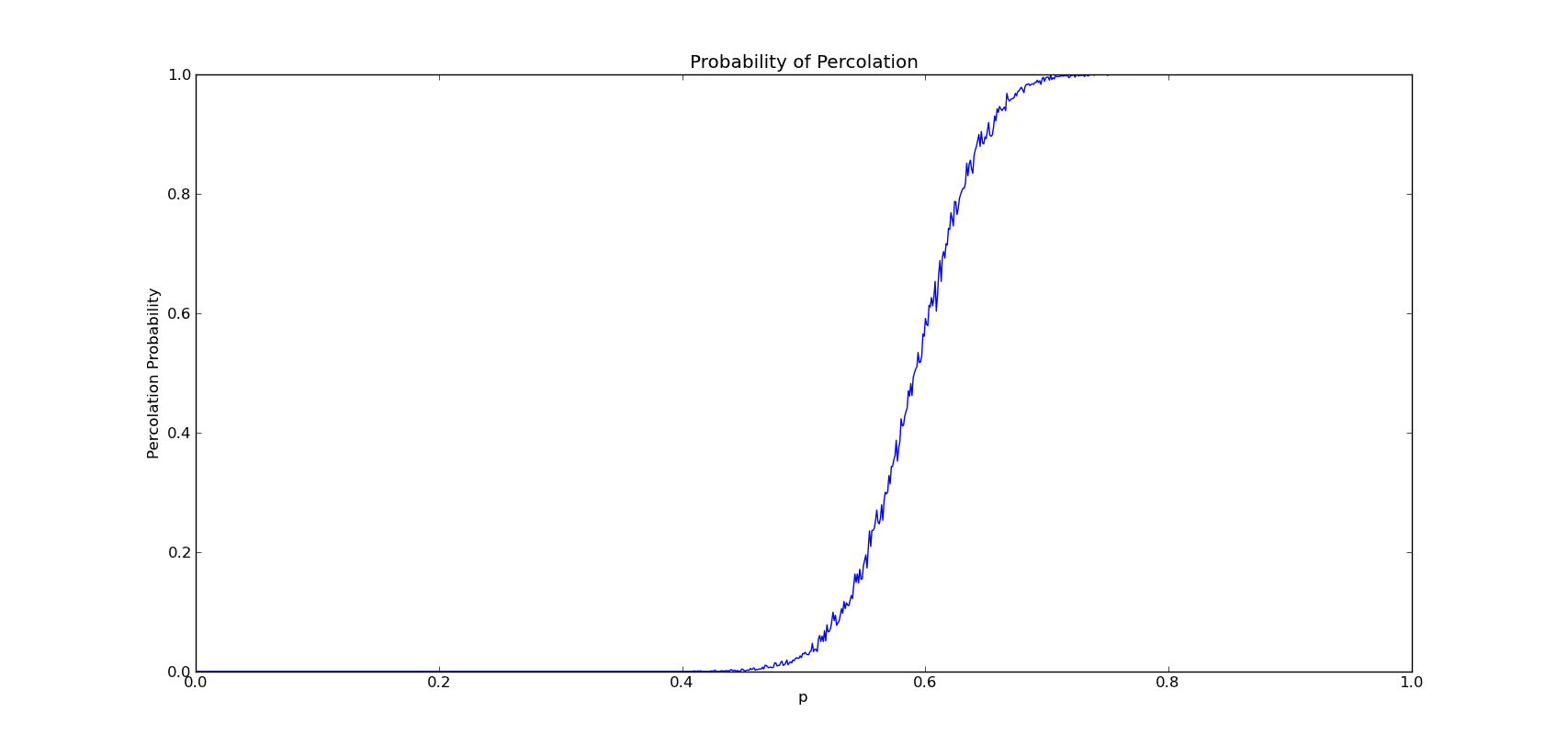
- N = 1000,M = 1000
- N = 1000,M = 100
- N = 1000,M = 10
- N = 100,M = 1000
- N = 100,M = 100
- N = 100,M = 10
1. N = 1000,M = 1000


6. N = 100,M = 10
7.其实也考虑了N = 10,M = 1000
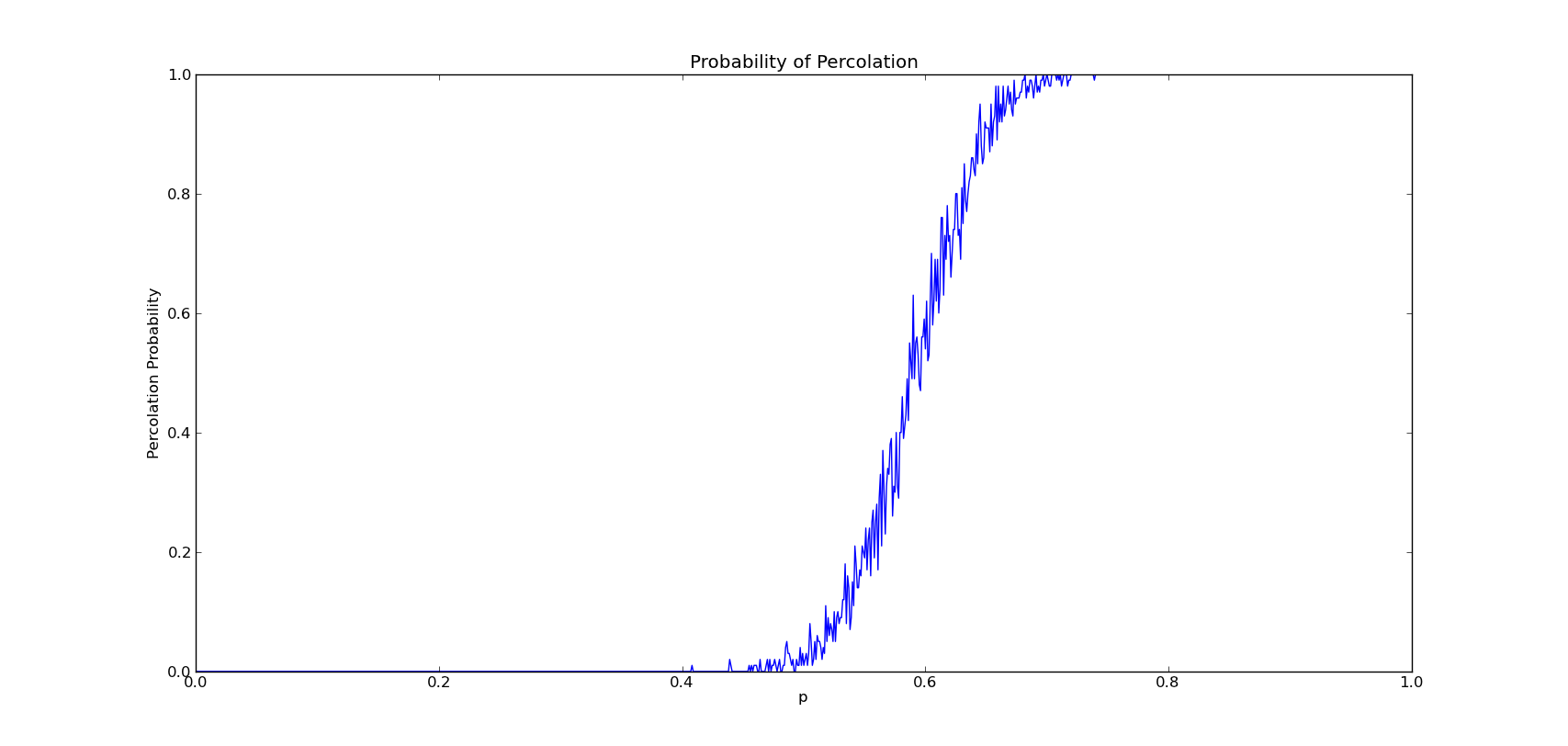
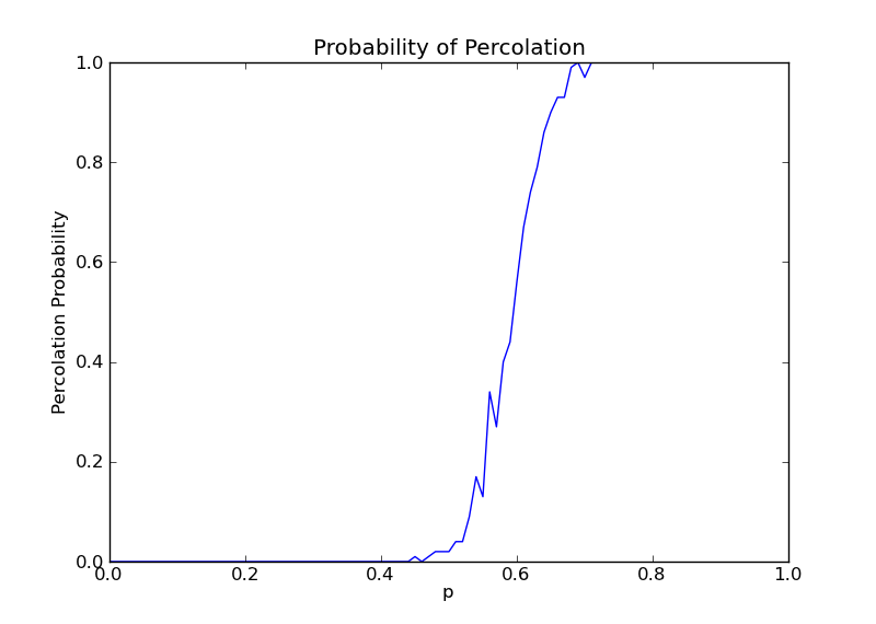
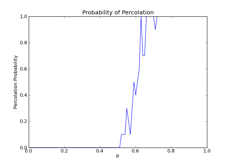
通过比较发现,当M过大时,曲线将出现不同幅度的波动,当N越小,这种现象越明显,这是因为网格其实由伪随机数生成,所以变化可能非常大。
当M过小时,曲线最终将变成直线的形式,这样隐藏于某一小段的p值的波动将被忽略,N越大,曲线将越光滑。
而且单是这个脚本的时间复杂度是O(MxN),约等于O(n²),这还没算水波算法的时间复杂度。
当有M和N中的一个值等于1000时,函数的执行时间大大增加,双1000的执行时间大约15分钟...
最终综上观察,我将会选择M,N=100,100的情况。