> ######因子分析
> pt<-read.csv("profile_telecom.csv")
> head(pt)
       ID cnt_call cnt_msg cnt_wei cnt_web
1 1964627       46      90      36      31
2 3107769       53       2       0       2
3 3686296       28      24       5       8
4 3961002        9       2       0       4
5 4174839      145       2       0       1
6 5068087      186       4       3       1
> library(psych)
> #用fa.parallel()确定主成分个数
> fa.parallel(pt,fa="both",n.iter = 100)###因子分析碎石图选转折点而不是特征根大于一

> #fa(pt,nfactors = ,rotate = "varimax",fm=""):fm提取因子方法有pa(主轴迭代)
> #、ml(最大似然)、wls(最小二乘)等方法
> ptfa<-fa(r=pt,nfactors = 2,rotate = "promax",fm="pa",scores = T)
> ptfa
Factor Analysis using method = pa
Call: fa(r = pt, nfactors = 2, rotate = "promax", scores = T, fm = "pa")
Standardized loadings (pattern matrix) based upon correlation matrix
PA1 PA2 h2 u2 com
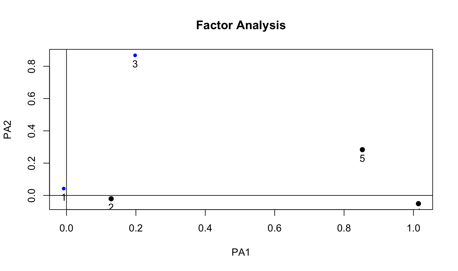
ID -0.01 0.04 0.0016 0.9984 1.1
cnt_call 0.13 -0.02 0.0148 0.9852 1.1
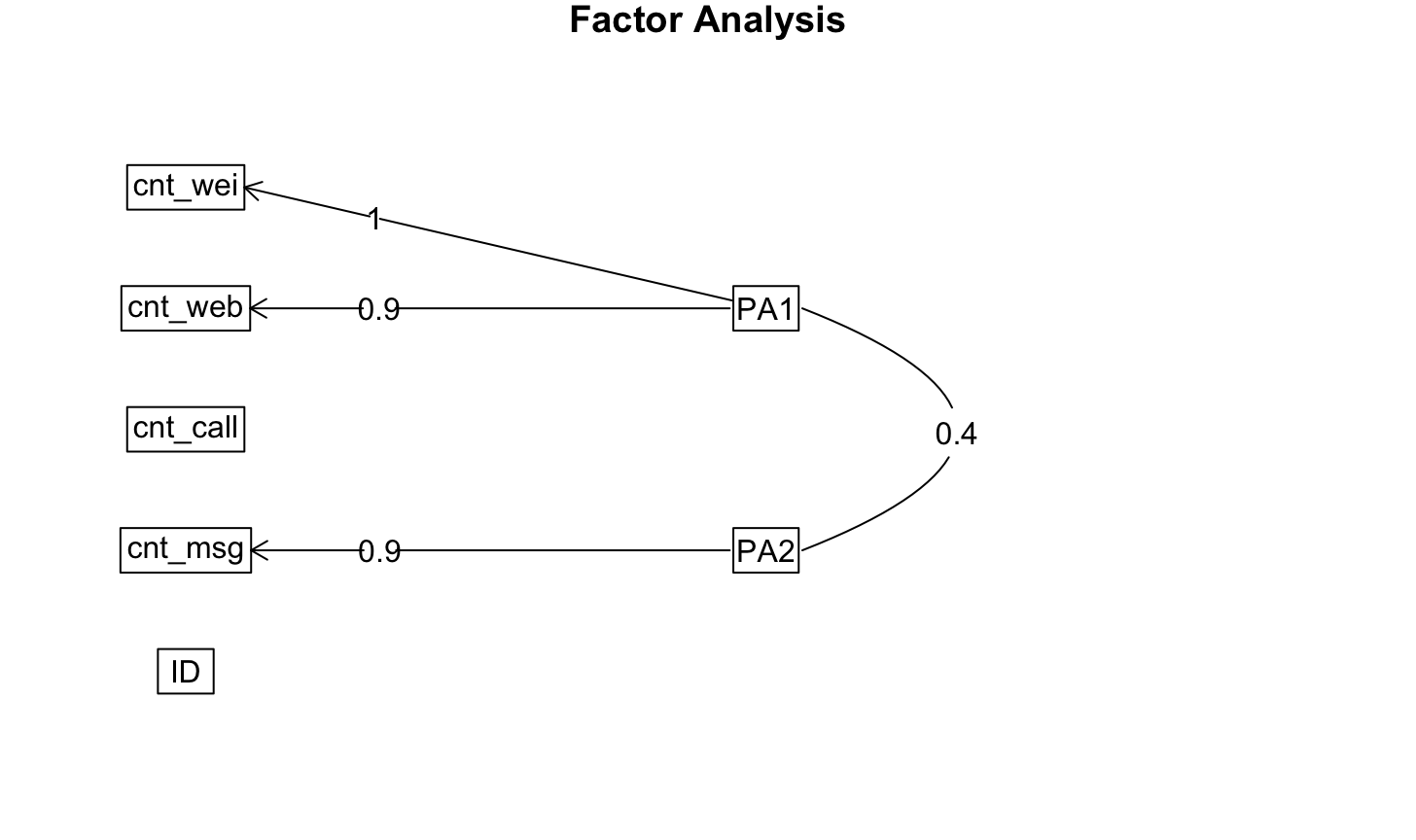
cnt_msg 0.20 0.87 0.9319 0.0681 1.1
cnt_wei 1.01 -0.05 0.9896 0.0104 1.0
cnt_web 0.85 0.28 1.0048 -0.0048 1.2
PA1 PA2
SS loadings 1.96 0.98
Proportion Var 0.39 0.20
Cumulative Var 0.39 0.59
Proportion Explained 0.67 0.33
Cumulative Proportion 0.67 1.00
With factor correlations of
PA1 PA2
PA1 1.00 0.41
PA2 0.41 1.00
Mean item complexity = 1.1
Test of the hypothesis that 2 factors are sufficient.
The degrees of freedom for the null model are 10 and the objective function was 5.01 with Chi Square of 2988.84
The degrees of freedom for the model are 1 and the objective function was 0.01
The root mean square of the residuals (RMSR) is 0.01
The df corrected root mean square of the residuals is 0.04
The harmonic number of observations is 600 with the empirical chi square 1.47 with prob < 0.23
The total number of observations was 600 with Likelihood Chi Square = 6.48 with prob < 0.011
Tucker Lewis Index of factoring reliability = 0.982
RMSEA index = 0.096 and the 90 % confidence intervals are 0.037 0.171
BIC = 0.09
Fit based upon off diagonal values = 1
Measures of factor score adequacy
PA1 PA2
Correlation of (regression) scores with factors 1 0.99
Multiple R square of scores with factors 1 0.98
Minimum correlation of possible factor scores 1 0.97
> tail(ptfa$scores)#看迭代结果的后五行
PA1 PA2
[595,] 1.7944781 8.40547805
[596,] 0.2931260 -0.72735784
[597,] -0.3431254 0.48556060
[598,] 3.0720057 -0.72170499
[599,] -0.1089760 0.06106985
[600,] -0.5381938 -0.47854547
> factor.plot(ptfa)
> ptsum<-cbind(ptpc,ptfa$scores)#和上期主成分分析的结果对比
> head(ptsum)
       ID cnt_call cnt_msg cnt_wei cnt_web        RC1        RC3        RC2        PA1
1 1964627       46      90      36      31  0.1952344  3.8712835 -0.3726676  1.1900638
2 3107769       53       2       0       2 -0.4219981 -0.6793516 -0.1552081 -0.5338358
3 3686296       28      24       5       8 -0.4194772  0.5202526 -0.5541321 -0.2507665
4 3961002        9       2       0       4 -0.2943034 -0.6714705 -0.8283602 -0.3536961
5 4174839      145       2       0       1 -0.5535192 -0.6802487  1.2451860 -0.6250782
6 5068087      186       4       3       1 -0.5413228 -0.6159420  1.8639601 -0.6259881
           PA2
1  4.036884424
2 -0.513818738
3  0.675144374
4 -0.007852624
5 -0.782894711
6 -1.046314108