壁虎书3 Classification

MNIST

　　fetch_openml returns the unsorted MNIST dataset, whereas fetch_mldata() returned the dataset sorted by target (the training set and the test set were sorted separately). 

import numpy as np

def sort_by_target(mnist):
    reorder_train = np.array(sorted([(target, i) for i, target in enumerate(mnist.target[:60000])]))[:, 1]
    reorder_test = np.array(sorted([(target, i) for i, target in enumerate(mnist.target[60000:])]))[:, 1]
    mnist.data[:60000] = mnist.data[reorder_train]
    mnist.target[:60000] = mnist.target[reorder_train]
    mnist.data[60000:] = mnist.data[reorder_test + 60000]
    mnist.target[60000:] = mnist.target[reorder_test + 60000]


from sklearn.datasets import fetch_openml

mnist = fetch_openml('mnist_784', version=1, cache=True)
mnist.target = mnist.target.astype(np.int8)  # fetch_openml() returns targets as strings
sort_by_target(mnist)

X, y = mnist['data'], mnist['target']
print(X.shape, y.shape)  # (70000, 784) (70000,)


import matplotlib.pyplot as plt

some_digit = X[36000]
some_digit_image = some_digit.reshape(28, 28)

plt.imshow(some_digit_image, cmap=plt.cm.binary, interpolation='nearest')
plt.axis('off')
plt.show()
print(y[36000])  # 5

　　split training set and test set. 

X_train, X_test, y_train, y_test = X[:60000], X[60000:], y[:60000], y[60000:]

　　shuffle the training set; this will guarantee that all cross-validation folds will be similar. moreover，some learning algorithms are sensitive to the order of the train instances，and they perform poorly if they get many similar instances in a row.

shuffle_index = np.random.permutation(60000)
X_train, y_train = X_train[shuffle_index], y_train[shuffle_index]

Training a Binary Classifier

　　create the target vectors for this classification task.

y_train_5 = (y_train == 5)
y_test_5 = (y_test == 5)

　　a good place to start is with a Stochastic Gradient Descent(SGD) classifier，using Scikit-Learn's SGDClassifier class. this classifier has the advantage of being capable of handling very large datasets efficiently. this is in part because SGD deals with training instances independently，one at a time(which also makes SGD well suited for online learning). 

from sklearn.linear_model import SGDClassifier

sgd_clf = SGDClassifier(max_iter=5, tol=-np.infty, random_state=42)
sgd_clf.fit(X_train, y_train_5)

some_digit = X[36000]
print(sgd_clf.predict([some_digit]))  # [ True]

Performance Measures

　　Evaluating a classifier is often significantly trickier than evaluating a regressor.

　　Measuring Accuracy Using Cross-Validation

　　Confusion Matrix

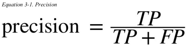
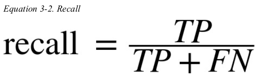
　　Precision and Recall

　　Precision/ Recall Tradeoff

　　The ROC Curve

measuring accuracy using cross-validation: 

　　occasionally you will need more control over the cross-validation process than what cross_val_score() and similar functions provide. in these cases，you can implement cross-validation yourself. the following code does roughly the same thing as the preceding cross_val_score(). 

from sklearn.model_selection import cross_val_score

scores = cross_val_score(sgd_clf, X_train, y_train_5, scoring='accuracy', cv=3)
print(scores)  # [0.96305 0.96515 0.967  ]

from sklearn.model_selection import StratifiedKFold
from sklearn.base import clone

skfolds = StratifiedKFold(n_splits=3, random_state=42)

for train_index, test_index in skfolds.split(X_train, y_train_5):
    clone_clf = clone(sgd_clf)  # 从意思上来看，是新模型从头开始训练
    X_train_folds = X_train[train_index]
    y_train_folds = y_train_5[train_index]
    X_test_fold = X_train[test_index]
    y_test_fold = y_train_5[test_index]

    clone_clf.fit(X_train_folds, y_train_folds)
    y_pred = clone_clf.predict(X_test_fold)
    n_correct = sum(y_pred == y_test_fold)
    print(n_correct / len(y_pred))

# 0.96305
# 0.96515
# 0.967

　　准确率都在96%以上，但别高兴太早，let's look at a very dumb classifier that just classifies every single image in the "not-5" class. 

from sklearn.base import BaseEstimator


class Never5Classifier(BaseEstimator):
    def fit(self, X, y=None):
        pass

    def predict(self, X):
        return np.zeros((len(X), 1), dtype=bool)


never_5_clf = Never5Classifier()
n_scores = cross_val_score(never_5_clf, X_train, y_train_5, scoring='accuracy', cv=3)
print(n_scores)  # [0.90765 0.90855 0.91275]

　　准确率也达到了90%以上。this is simply because only about 10% of the images are 5s，so if always guess that an image is not a 5，you will be right about 90%.  Beats Nostradamus. 

　　this demonstrates why accuracy is generally not the preferred performance measure for classifiers，especially when you are dealing with skewed datasets(i.e., when some classes are much more frequent than others). 

confusion matrix: 

　　a much better way to evaluate the performance of a classifier is to look at the confusion matrix. the general idea is to count the number of times instances of class A are classified as class B. for example，to know the number of times the classifier consused images of 5s with 3s，you would look in the fifth row and third column of the confusion matrix. 

　　to compute the confusion matrix，you first need to have a set of predictions，so they can be compared to the actual targets. you can use the cross_val_predict() function. 

　　just like the cross_val_score() function，cross_val_predict() performs K-fold cross-validation，but instead of returning the evaluation scores，it return the predictions made on each test fold. this means that you get a clean perdition for each instance in the training set("clean" meaning that the prediction is made by a model that never saw the data during training). 

from sklearn.model_selection import cross_val_predict
from sklearn.metrics import confusion_matrix

y_train_pred = cross_val_predict(sgd_clf, X_train, y_train_5, cv=3)
matrix = confusion_matrix(y_train_5, y_train_pred)
print(matrix)

# [[53896   683]
#  [ 1583  3838]]

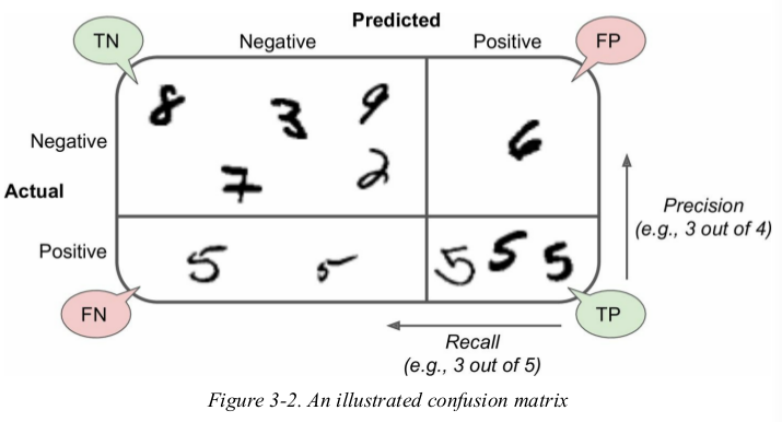
　　each row in a confusion matrix represents an actual class，while each column represents a predicted class. the first row of this matrix considers non-5 images(the negative class): 53896 of them were correctly classified as non-5s(they are called true negatives)，while the remaining 683 were wrongly classified as 5s(false positives). the second row considers the images of 5s(the positive class): 1583 were wrongly classified as non-5s(false negatives)，while the remaining 3838 were correctly classified as 5s(true positives). a perfect classifier would have only true positives and true negatives，so its confusion matrix would have nonzero values only on its main diagonal. 

　　a more concise metric to look at is the accuracy of  the positive predictions，this is called the precision of the classifier.

　　

　　another metric named recall，also called sensitivity or true positive rate(TPR): this is the radio of positive instances that are correctly detected by the classifier.

　　

　　precision and recall 示意图

precision and recall: 

　　Scikit-Learn provides several functions to compute classifier metrics，including precision and recall.

from sklearn.metrics import precision_score, recall_score

score = precision_score(y_train_5, y_train_pred)
print(score)  # 0.7316459939658062
score = recall_score(y_train_5, y_train_pred)
print(score)  # 0.805201992252352

　　now the 5-detector does not look as shiny as it did when you looked at its accuracy. 

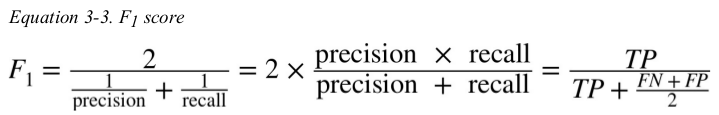
　　it is often convenient to combine precision and recall into a single metric called the F1 score，in particular if you need a simple way to compare two classifiers. the F1 score is the harmonic mean of precision and recall，the harmonic mean given much more weight to low values. as a result，the classifier will only get a high F1 score if both precision and recall are high.

　　

from sklearn.metrics import f1_score

f1_score = f1_score(y_train_5, y_train_pred)
print(f1_score)  # 0.8004653868528214

　　the F1 score favours classifiers that have similar precision and recall. this is not always what you want: in some contexts you mostly care about precision，and in  other contexts you really care about recall. for example，if you trained a classifier to detect videos that are safe for kids，you would probably prefer a classifier that reject many good videos(low recall) but keeps only safe ones(high precision). on the other hand，suppose you train a classifier to detect shoplifters on surveillance images: it is probably fine if your classifier has only 30% precision as long as it has 99% recall. 

　　unfortunately，you can't have it both ways: increasing precision reduces recall，and vice versa. this is called the precision/ recall tradeoff. 

precision/ recall tradeoff: 

　　the approach that the SGDClassifier makes its classification decisions. for each instanc，it computes a score based on a decision function，and if that score is greater than a threshold，it assigns the instance to the positive class，or else it assigns it to the negative class. 

　　

　　Scikit-Learn doesn't let you set the threshold directly，but it gives you access to the decision scores that it uses to make prediction. you can call its decision_function() method，which returns a score for each instance，and then make predictions based on those scores using any threshold you want: 

y_scores = sgd_clf.decision_function([some_digit])
print(y_scores)  # [44427.85526221]
threshold = 0
y_some_digit_pred = (y_scores > threshold)
print(y_some_digit_pred)  # [ True]

　　so how can you decide which threshold to use？first，you need to get the scores of all instances in the training set using the cross_val_predict() function again，but this time specifying that you want it to return decision scores instead of predictions.  then，with these scores you can compute precision and recall for all possible thresholds using the precision_recall_curve() function. finally，you can plot precision and recall as functions of the the threshold value using Matplotlib. 

from sklearn.model_selection import cross_val_predict
from sklearn.metrics import precision_recall_curve
import matplotlib.pyplot as plt
# 要求sgd_clf 有decision_function方法
y_scores = cross_val_predict(sgd_clf, X_train, y_train_5, cv=3, method='decision_function')

precisions, recalls, thresholds = precision_recall_curve(y_train_5, y_scores)

def plot_precision_recall_vs_threshold(precisions, recalls, thresholds):
    plt.plot(thresholds, precisions[:-1], 'b--', label='Precision')
    plt.plot(thresholds, recalls[:-1], 'g-', label='Recall')
    plt.xlabel('Thresholds')
    plt.legend(loc='upper left')
    plt.ylim([0, 1])

plot_precision_recall_vs_threshold(precisions, recalls, thresholds)
plt.show()

　　

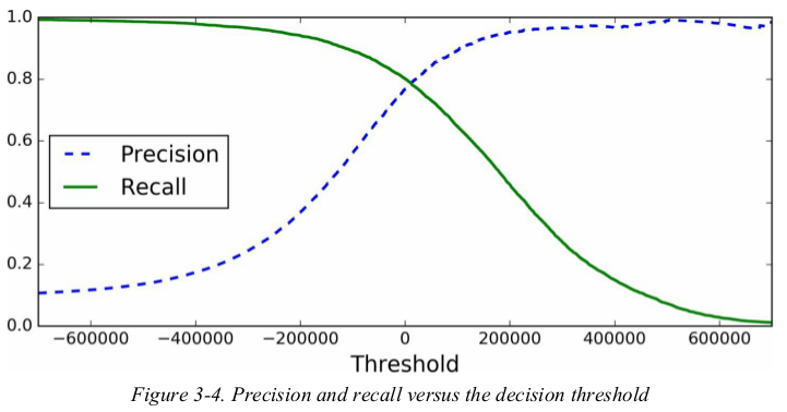
　　the precision curve is bumpier than the recall curve in Figure3-4. the reason is that precision may sometimes go down when you raise the threshold(although in generally it will go up). to understand why，look back at Figure3-3 and move the central threshold just one digit to the right: precision goes from 4/5(80%) down to 3/4(75%). on the other hand，recall can only go down when the threshold is increased. 

　　now you can simply select the threshold value that gives you the best precision/ recall tradeoff for your task. another way to select a good precision/ recall tradeoff is to plot precision directly against recall. 

　　

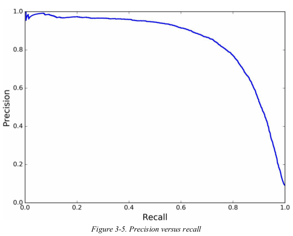
　　you can see that precision really starts to fall sharply around 80% recall. you will probably want to select a precision/ recall tradeoff just before that drop. 

from sklearn.metrics import precision_score, recall_score

y_train_pred_90 = (y_scores > 70000)
print(precision_score(y_train_5, y_train_pred_90))  # 0.9225788288288288
print(recall_score(y_train_5, y_train_pred_90))  # 0.604501014572957

the ROC curve: 

　　the receive operating characteristic(ROC) curve is another common tool used with binary classifier. it is very similar to the precision/ recall curve，but instead of plotting precision versus recall，the ROC curve plots the true positive rate(another name for recall) against the false positive rate. the FPR is the ratio of negative instances that are incorrectly classified as positive. it is equal to one minute the true negative rate，which is the radio of negative instances that are correctly classified as negative. the TNR is also called specificity. hence，the ROC curve plots sensitivity(recall) versus 1 - specificity. 

　　to plot the ROC curve，you first need to compute the TPR and FPR for various threshold values，using the roc_curve() function. 

from sklearn.metrics import roc_curve

fpr, tpr, thresholds = roc_curve(y_train_5, y_scores)

def plot_roc_curve(fpr, tpr, label=None):
    plt.plot(fpr, tpr, linewidth=2, label=label)
    plt.plot([0, 1], [0, 1], 'k--')
    plt.axis([0, 1, 0, 1])
    plt.xlabel('False Positive Rate')
    plt.ylabel('True Positive Rate')

plot_roc_curve(fpr, tpr)
plt.show()

　　

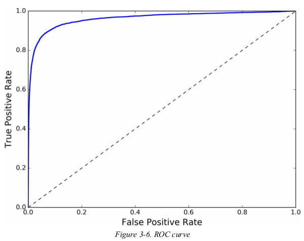
　　once again there is a tradeoff: the higher the recall(TPR)，the more false positive(FPR). the dotted line represents the ROC curve of a purely random classifier；a good classifier stays as far away from that line as possible. 

　　one way to compare classifiers is to measure the area under the curve(AUC)，a perfect classifier will have a ROC AUC equal 1，whereas a purely random classifier will have a ROC AUC equal to 0.5. Scikit-Learn provides a function to compute the ROC AUC. 

from sklearn.metrics import roc_auc_score

print(roc_auc_score(y_train_5, y_scores))  # 0.9607201080651024

　　since the ROC curve is so similar to the precision/ recall(or PR) curve，how to decide which one to use. you should prefer the PR curve whenever the positive class is rare or when you care more about the false positive than the false negative，and the ROC curve otherwise.  但是举的例子好像有问题╮(╯▽╰)╭？

　　

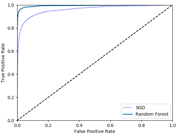
　　let's train a RandomForestClassifier and compare its ROC curve and ROC AUC score to the SGDClassifier. first，you need to get scores for each instance in the training set. But due to the way it works，the RandomForestClassifier class does not have a decision_function() method. but it has a predict_proba() method. the predict_proba() method returns an array containing a row per instance and a column per class，each containing the probability that the given instance belongs to the given class. 

　　but to plot a ROC curve，you need scores，not probabilities. a simple solution is to use the positive class's probability as the score. 

from sklearn.ensemble import RandomForestClassifier

forest_clf = RandomForestClassifier(n_estimators=10, random_state=42)
y_probas_forest = cross_val_predict(forest_clf, X_train, y_train_5, cv=3, method='predict_proba')

y_scores_forest = y_probas_forest[:, 1]
fpr_forest, tpr_forest, thresholds_forest = roc_curve(y_train_5, y_scores_forest)

plt.plot(fpr, tpr, 'b:', label='SGD')
plot_roc_curve(fpr_forest, tpr_forest, 'Random Forest')
plt.legend(loc='lower right')
plt.show()

print(roc_auc_score(y_train_5, y_scores_forest))  # 0.9921660581128391

　　

Multiclass Classification

　　some algorithms(such as Random Forest classifiers or naive Bayes classifiers) are capable of handling multiple classes directly. others(such as Support Vector Machine classifiers or Linear classifiers) are strictly binary classifiers. however，there are various strategies that you can use to perform multiclass classification using multiclass binary classifiers. 

　　for example，one way to create a system that can classify the digit images into 10 classes(from 0 to 9) is to train 10 binary classifiers，one for each digit. then when you want to classify an image，you get decision score from each classifier for that image and select the class whose classifier outputs the highest score. this is called the one-versus-all(OvA) strategy. 

　　another strategy is to train a binary classifier for every pair of digits: one to distinguish 0s and 1s，another to distinguish 0s and 2s，another for 1s and 2s，and so on. this is called one-versus-one(OvO) strategy. if there are N classes，you need to train N × (N - 1) / 2 classifiers.  the main advantage of OvO is that each classifier only needs to be trained on the part of the training set for the two classes that it must distinguish. 

　　some algorithms(such as Support Vector Machine classifiers) scale poorly with the size of the training set，so for these algorithms OvO is preferred since it is faster to train many classifiers on small training set than training few classifiers on large training set. for most binary classification algorithms，however，OvA is preferred. 

　　Scikit-Learn detects when you try to use a binary classification algorithm for a multiclass classification task，and it automatically runs OvA(except for SVM classifier for which it uses OVO).

from sklearn.linear_model import SGDClassifier

sgd_clf = SGDClassifier(max_iter=5, tol=-np.infty, random_state=42)
sgd_clf.fit(X_train, y_train)
print(sgd_clf.predict([some_digit]))  # [5]

some_digit_scores = sgd_clf.decision_function([some_digit])
print(some_digit_scores)
# [[-138039.11010526 -345962.50027719 -328025.06610149  -65114.66126866
#   -395522.41437973  107953.56128123 -791140.93654843 -247782.51116479
#   -684172.27642421 -576428.25618674]]
print(sgd_clf.classes_)  # [0 1 2 3 4 5 6 7 8 9]

　　if you want to force Scikit-Learn to use one-versus-one or one-versus-all，you can use the OneVsOneClassifier or OneVsRestClassifier classes. simply create an instance and pass a binary classifier to its constructor. 

from sklearn.multiclass import OneVsOneClassifier

sgd_clf = SGDClassifier(max_iter=5, tol=-np.infty, random_state=42)
ovo_clf = OneVsOneClassifier(sgd_clf)
ovo_clf.fit(X_train, y_train)
print(ovo_clf.predict([some_digit]))  # [5]
print(len(ovo_clf.estimators_))  # 45个

　　training a RandomForestClassifier is just as easy. this time Scikit-Learn did not have to run OvA or OVO because Random Forest classifiers can directly classify instances into multiple classes. you can call predict_proba() to get the list of probabilities that the classifier assigned to each instance for each class. 

from sklearn.ensemble import RandomForestClassifier

forest_clf = RandomForestClassifier(n_estimators=10, random_state=42)
forest_clf.fit(X_train, y_train)
print(forest_clf.predict([some_digit]))  # [5]

print(forest_clf.predict_proba([some_digit]))
# [[0.  0.  0.  0.1 0.  0.8 0.  0.  0.1 0. ]]

　　evaluate the SGDClassifier's accuracy using the cross_val_scores() function. 

print(cross_val_score(sgd_clf, X_train, y_train, scoring='accuracy', cv=3))
# [0.8659768  0.85914296 0.84822723]

　　simply scaling the inputs increases accuracy above 90%.

from sklearn.preprocessing import StandardScaler

std_scale = StandardScaler()
X_train_std = std_scale.fit_transform(X_train)
print(cross_val_score(sgd_clf, X_train_std, y_train, cv=3, scoring='accuracy'))
# [0.91136773 0.90739537 0.91218683]

Error Analysis

　　here，assume that you have found a promising model and want to find ways to improve it. one way to do this is to analyze the types of errors it makes. 

　　first，you can look at the confusion matrix. 与二分类时一样。

from sklearn.model_selection import cross_val_predict
from sklearn.metrics import confusion_matrix

y_train_pred = cross_val_predict(sgd_clf, X_train_scaled, y_train, cv=3)
conf_mx = confusion_matrix(y_train, y_train_pred)
print(conf_mx)
# [[5728    4   29    7    9   55   41   10   36    4]
#  [   1 6493   41   24    6   39    7   12  106   13]
#  [  53   36 5327  108   67   27   98   57  169   16]
#  [  48   43  139 5353    1  227   42   60  119   99]
#  [  15   30   42    9 5364    9   58   33   63  219]
#  [  68   43   32  192   68 4591  114   28  185  100]
#  [  31   27   49    1   40  102 5614    9   45    0]
#  [  24   20   69   27   53   11    5 5807   15  234]
#  [  49  165   67  169   15  153   62   25 4993  153]
#  [  46   35   29   90  160   32    2  198   67 5290]]

　　that's a lot of numbers. it's often more convenient to look at an image representative of the confusion matrix，using Matplotlib's matshow() function. 

plt.matshow(conf_mx, cmap=plt.cm.gray)
plt.show()

　　

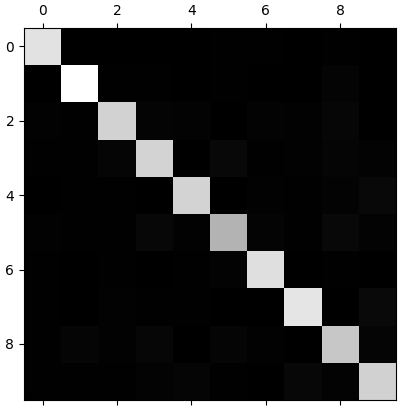
　　the 5s look slightly darker than the other digits，which could mean that there are fewer images of 5s in the datasets or that the classifier does not performs as well on 5s as on other digits. in fact，you can verify that both are the case. 

　　focus the plot on the errors. first，you need to divide each value in the confusion matrix by the number of images in the corresponding class，so you can compare error rates instead of absolute number of errors. then，fill the diagonal with zeros to keep only the errors. 

row_sums = conf_mx.sum(axis=1, keepdims=True)
norm_conf_mx = conf_mx / row_sums

np.fill_diagonal(norm_conf_mx, 0)
plt.matshow(norm_conf_mx, cmap=plt.cm.gray)
plt.show()

　　

　　the column for classes 8 and 9 are quite bright，which tells you that many images get misclassified as 8s or 9s. similarly，the rows for classes 8 and 9 are also quite bright，telling you that 8s and 9s are often confused with other digits. conversely，some rows are pretty dark，such as row 1: this means that most 1s are classified correctly. 

　　analyzing the confusion matrix can often give you insights on ways to improve your classifier. Looking at this plot，it seems that your efforts should be spent on improving classification of 8s and 9s，as well as fixing the specific 3/ 5 confusion. for example，you could try to gather more training data for these digits. or you could engineer new features that would help the classifier——for example，writing an algorithm to count the number of closed loops(e.g., 8 has two，6 has one，5 has none). or you could preprocess the images(e.g., using Scikit-Learn，Pillow，or OpenCV) to make some patterns stand out more，such as closed loops. 

　　analyzing individual errors can also be a good way to gain insights on what your classifier is doing and why it is failing，but it is more difficult and time-consuming. 

c1_a, c1_b = 3, 5
X_aa = X_train[(y_train == c1_a) & (y_train_pred == c1_a)]
X_ab = X_train[(y_train == c1_a) & (y_train_pred == c1_b)]
X_ba = X_train[(y_train == c1_b) & (y_train_pred == c1_a)]
X_bb = X_train[(y_train == c1_b) & (y_train_pred == c1_b)]

def plot_digits(instances, images_per_row=10, **options):
    size = 28
    images_per_row = min(len(instances), images_per_row)
    images = [instance.reshape(size, size) for instance in instances]
    n_rows = (len(instances) - 1) // images_per_row + 1
    row_images = []
    n_empty = n_rows * images_per_row - len(instances)
    images.append(np.zeros((size, size * n_empty)))
    for row in range(n_rows):
        rimages = images[row * images_per_row : (row + 1) * images_per_row]
        row_images.append(np.concatenate(rimages, axis=1))
    image = np.concatenate(row_images, axis=0)
    plt.imshow(image, cmap=plt.cm.binary, **options)
    plt.axis("off")

plt.figure(figsize=(8, 8))
plt.subplot(221); plot_digits(X_aa[:25], images_per_row=5)
plt.subplot(222); plot_digits(X_ab[:25], images_per_row=5)
plt.subplot(223); plot_digits(X_ba[:25], images_per_row=5)
plt.subplot(224); plot_digits(X_bb[:25], images_per_row=5)
plt.show()

　　

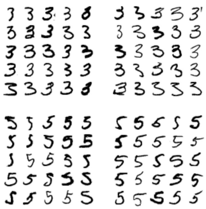
　　some of digits that the classifier gets wrong(i.e., in the bottom-left and top-right blocks) are so badly written that even a human would have trouble classifying them(e.g., the 5 on the eighth row and first column truly looks like a 3). however，most misclassified images seem like obvious errors to us. the reason is that we used a simple SGDClassifier，which is a linear model. all it does is assign a weight per class to each pixel，and when it sees a new image it just sums up the weighted pixel intensities to get a score for each class. so since 3s and 5s differ only by a few pixels，this model will easily confuse them. 

　　the main difference between 3s and 5s is the position of the small line that joins the top line to the bottom arc. if you draw a 3 with the junction slightly shifted to the left，the classifier might classify it as a 5，and vice versa. in other words，this classifier is quite sensitive to image shifting and rotation. so one way to reduce the 3/ 5 confusion would be to preprocess the images to ensure that they are well centered and not too rotated. this will probably help reduce other errors as well. 

Multilabel Classification

　　for example，consider a face-recognition classifier: what should it do if it recognizes several people on the same picture？of course it should attach one label per person it recognizes. such a classification system that outputs multiple binary labels is called a multilabel classification system. 

　　the KNeighborsClassifier instance supports multilabel classification，but not all classifiers do. 

from sklearn.neighbors import KNeighborsClassifier

y_train_large = (y_train >= 7)
y_train_odd = (y_train % 2 == 1)
y_multilabel = np.c_[y_train_large, y_train_odd]

knn_clf = KNeighborsClassifier()
knn_clf.fit(X_train, y_multilabel)

print(knn_clf.predict([some_digit]))  # [[False  True]]

　　there are many ways to evaluate a multilabel classifier. for example，one approach is to measure the F1 score for each individual label，then simply compute the average score. 

from sklearn.metrics import f1_score

y_train_knn_pred = cross_val_predict(knn_clf, X_train, y_train, cv=3)
print(f1_score(y_train, y_train_knn_pred, average='macro'))  # 0.9687059409209977

　　this assumes that all labels are equally important，which may not be the case. in particular，if you have many more pictures of Alice than of Bob or Charlie，you may want to give more weight to the classifier's score on pictures of Alice. one simple option is to give each label a weight equal to its support(i.e., the number of instances with that target label). to do this，simply set average='weighted' in the preceding code. 

Multioutput Classification

　　it is simply a generalization of multilabel classification where each label can be multiclass(i.e., it can have more than two possible values). 

　　to illustrate this，let's build a system that removes noise from images. 

noise = np.random.randint(0, 100, (len(X_train), 784))
X_train_mod = X_train + noise
noise = np.random.randint(0, 100, (len(X_test), 784))
X_test_mod = X_test + noise
y_train_mod = X_train
y_test_mod = X_test

def plot_digit(data):
    image = data.reshape(28, 28)
    plt.imshow(image, cmap=plt.cm.binary, interpolation="nearest")
    plt.axis("off")
#
# some_index = 5500
# plt.subplot(121)
# plot_digit(X_test_mod[some_index])
# plt.subplot(122)
# plot_digit(y_test_mod[some_index])
# plt.show()

knn_clf = KNeighborsClassifier()
knn_clf.fit(X_train_mod, y_train_mod)
clean_digit = knn_clf.predict([X_test_mod[5500]])
plot_digit(clean_digit)
plt.show()

Exercises

　　1. build a classifier for the MNIST dataset that achieves over 97% accuracy on the test set. 　　Hint: the KNeighborsClassifier works quite well for this task；you just need to find good hyperparameter values (try a grid search on the weights and n_neighbors hyperparameters). 

from sklearn.model_selection import GridSearchCV
from sklearn.metrics import accuracy_score

param_grid = {'n_neighbors': [3, 4, 5], 'weights': ['uniform', 'distance']}
knn_clf = KNeighborsClassifier()
grid_search = GridSearchCV(knn_clf, param_grid, cv=5, verbose=3, n_jobs=-1)
grid_search.fit(X_train, y_train)
print(grid_search.best_params_)
print(grid_search.best_score_)
print(grid_search.cv_results_)

y_pred = grid_search.predict(X_test)
print(accuracy_score(y_test, y_pred))

　　2. data augmentation or training set expansion: 

　　Write a function that can shift an MNIST image in any direction (left, right, up, or down) by one pixel. Then, for each image in the training set, create four shifted copies (one per direction) and add them to the training set. Finally, train your best model on this expanded training set and measure its accuracy on the test set.

　　You should observe that your model performs even better now! This technique of artificially growing the training set is called data augmentation or training set expansion. 

from scipy.ndimage.interpolation import shift

def shift_image(image, dx, dy):
    image = image.reshape((28, 28))
    shifted_image = shift(image, [dy, dx], cval=0, mode='constant')
    return shifted_image.reshape([-1])

image = X_train[1000]
shifted_image_down = shift_image(image, 0, 5)
shifted_image_left = shift_image(image, -5, 0)

# plt.figure(figsize=(12, 3))
# plt.subplot(131)
# plt.title('Original', fontsize=14)
# plt.imshow(image.reshape(28, 28), interpolation='nearest', cmap='Greys')
# plt.subplot(132)
# plt.title('Shifted down', fontsize=14)
# plt.imshow(shifted_image_down.reshape(28, 28), interpolation='nearest', cmap='Greys')
# plt.subplot(133)
# plt.title('Shifted left', fontsize=14)
# plt.imshow(shifted_image_left.reshape(28, 28), interpolation='nearest', cmap='Greys')
# plt.show()


from sklearn.neighbors import KNeighborsClassifier
from sklearn.metrics import accuracy_score

X_train_augmented = [image for image in X_train]
y_train_augmented = [label for label in y_train]

for dx, dy in ((1, 0), (-1, 0), (0, 1), (0. -1)):
    for image, label in zip(X_train, y_train):
        X_train_augmented.append(shift_image(image, dx, dy))
        y_train_augmented.append(label)

X_train_augmented = np.array(X_train_augmented)
y_train_augmented = np.array(y_train_augmented)

shuffle_idx = np.random.permutation(len(X_train_augmented))
X_train_augmented = X_train_augmented[shuffle_idx]
y_train_augmented = y_train_augmented[shuffle_idx]

knn_clf = KNeighborsClassifier(**grid_search.best_params_)
knn_clf.fit(X_train_augmented, y_train_augmented)
y_pred = knn_clf.predict(X_test)
print(accuracy_score(y_test, y_pred))