author:yangjing
date:2018-10-24
KMeans
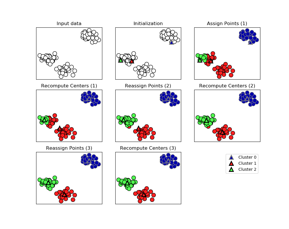
1.Process:
The algorithm alternates between two steps:1)assigning each data point to the closet cluter center,2)setting each cluster center as the mean of data points that are assigned to it.The algorithm is finished when the assignment of instances to cluster no longer changed.
2.Drawback
- Inertia makes the assumption that clusters are convex and isotropic, which is not always the case. It responds poorly to elongated clusters, or manifolds with irregular shapes.(对于凸型数据有很好的聚类效果,但对于细长的数据或是流型等不规则形状数据可能效果不是很理想)
- Inertia is not a normalized metric: we just know that lower values are better and zero is optimal. But in very high-dimensional spaces, Euclidean distances tend to become inflated . Running a dimensionality reduction algorithm such as PCA prior to k-means clustering can alleviate this problem and speed up the computations.(对于高维空间,一般先使用PCA或NMF降维,再做kmeans聚类)
- Relied on a random initialiation,which means the outcome of algorithm depends on a random seed.
3.code
print(__doc__)
from time import time
import numpy as np
import matplotlib.pyplot as plt
from sklearn import metrics
from sklearn.cluster import KMeans
from sklearn.datasets import load_digits
from sklearn.decomposition import PCA
from sklearn.preprocessing import scale
np.random.seed(42)
digits = load_digits()
data = scale(digits.data)
n_samples, n_features = data.shape
n_digits = len(np.unique(digits.target))
labels = digits.target
sample_size = 300
print("n_digits: %d, n_samples %d, n_features %d"
% (n_digits, n_samples, n_features))
print(82 * '_')
print('init time inertia homo compl v-meas ARI AMI silhouette')
def bench_k_means(estimator, name, data):
t0 = time()
estimator.fit(data)
print('%-9s %.2fs %i %.3f %.3f %.3f %.3f %.3f %.3f'
% (name, (time() - t0), estimator.inertia_,
metrics.homogeneity_score(labels, estimator.labels_),
metrics.completeness_score(labels, estimator.labels_),
metrics.v_measure_score(labels, estimator.labels_),
metrics.adjusted_rand_score(labels, estimator.labels_),
metrics.adjusted_mutual_info_score(labels, estimator.labels_),
metrics.silhouette_score(data, estimator.labels_,
metric='euclidean',
sample_size=sample_size)))
bench_k_means(KMeans(init='k-means++', n_clusters=n_digits, n_init=10),
name="k-means++", data=data)
bench_k_means(KMeans(init='random', n_clusters=n_digits, n_init=10),
name="random", data=data)
# in this case the seeding of the centers is deterministic, hence we run the
# kmeans algorithm only once with n_init=1
pca = PCA(n_components=n_digits).fit(data)
bench_k_means(KMeans(init=pca.components_, n_clusters=n_digits, n_init=1),
name="PCA-based",
data=data)
print(82 * '_')
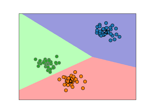
# #############################################################################
# Visualize the results on PCA-reduced data
reduced_data = PCA(n_components=2).fit_transform(data)
kmeans = KMeans(init='k-means++', n_clusters=n_digits, n_init=10)
kmeans.fit(reduced_data)
# Step size of the mesh. Decrease to increase the quality of the VQ.
h = .02 # point in the mesh [x_min, x_max]x[y_min, y_max].
# Plot the decision boundary. For that, we will assign a color to each
x_min, x_max = reduced_data[:, 0].min() - 1, reduced_data[:, 0].max() + 1
y_min, y_max = reduced_data[:, 1].min() - 1, reduced_data[:, 1].max() + 1
xx, yy = np.meshgrid(np.arange(x_min, x_max, h), np.arange(y_min, y_max, h))
# Obtain labels for each point in mesh. Use last trained model.
Z = kmeans.predict(np.c_[xx.ravel(), yy.ravel()])
# Put the result into a color plot
Z = Z.reshape(xx.shape)
plt.figure(1)
plt.clf()
plt.imshow(Z, interpolation='nearest',
extent=(xx.min(), xx.max(), yy.min(), yy.max()),
cmap=plt.cm.Paired,
aspect='auto', origin='lower')
plt.plot(reduced_data[:, 0], reduced_data[:, 1], 'k.', markersize=2)
# Plot the centroids as a white X
centroids = kmeans.cluster_centers_
plt.scatter(centroids[:, 0], centroids[:, 1],
marker='x', s=169, linewidths=3,
color='w', zorder=10)
plt.title('K-means clustering on the digits dataset (PCA-reduced data)
'
'Centroids are marked with white cross')
plt.xlim(x_min, x_max)
plt.ylim(y_min, y_max)
plt.xticks(())
plt.yticks(())
plt.show()