3. Matplotlib图像属性控制
3.1 色彩和样式(通过help(plt.plot)来查看符号对应含义)
plt.plot(listKOindex, listKO, 'g--') # 绿色虚线
plt.plot(listKOindex, listKO, 'rD') # 红色钻石
3.2 文字:为图、横轴和纵轴加标题
plt.title('Stock Statistics of Coca-Cola') # 图标题
plt.xlabel('Month') # 横轴标题
plt.ylabel('Average Close Price') # 纵轴标题
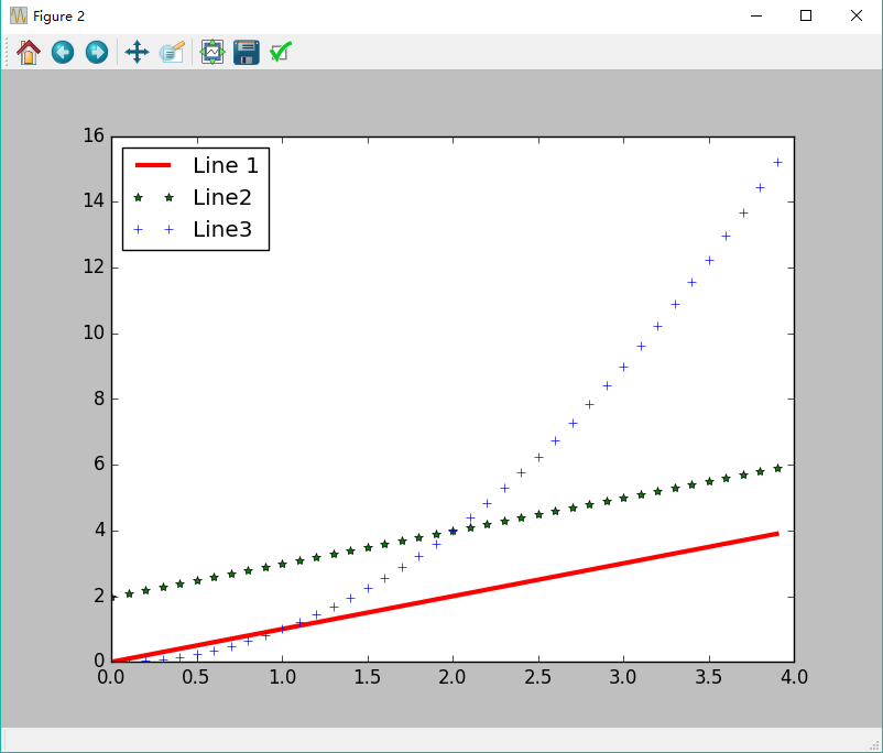
3.3 其他属性(figure(figsize=(8,6), dpi=50))(pl.legend(loc='upper left'))


# -*- coding: utf-8 -*-
"""
Created on Tue Jan 24 13:07:01 2017

@author: Wayne
"""

import pylab as pl
import numpy as np
pl.figure(figsize=(8,6), dpi=100)  # 创建一个8*6 点(point)的图,并设置分辨率为100
t = np.arange(0.,4.,0.1)
pl.plot(t,t,color='red',linestyle='-',linewidth=3,label='Line 1')
pl.plot(t,t+2,color='green',linestyle='',marker='*',linewidth=3,label='Line2')
pl.plot(t,t**2,color='blue',linestyle='',marker='+',linewidth=3,label='Line3')
pl.legend(loc='upper left')  # 图例放在左上角
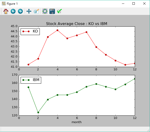
3.4 子图 subplot:将KO公司和IBM公司近一年来股票收盘价的月平均价绘制在一张图中
# -*- coding: utf-8 -*-
"""
Created on Tue Jan 24 13:07:01 2017

@author: Wayne
"""

from matplotlib.finance import quotes_historical_yahoo_ochl
from datetime import date, datetime
import time
import pandas as pd
import matplotlib.pylab as pl
today = date.today()
start = (today.year-1, today.month, today.day)
quotes1 = quotes_historical_yahoo_ochl('KO', start, today)
quotes2 = quotes_historical_yahoo_ochl('IBM', start, today)
fields = ['date','open','close','high','low','volume']
list1 = []
list2 = []
for i in range(0,len(quotes1)):
    x = date.fromordinal(int(quotes1[i][0]))
    y = datetime.strftime(x,'%Y-%m-%d')
    list1.append(y)
for i in range(0,len(quotes2)):
    x = date.fromordinal(int(quotes2[i][0]))
    y = datetime.strftime(x,'%Y-%m-%d')
    list2.append(y)

quoteskodf1 = pd.DataFrame(quotes1, index = list1, columns = fields)
quoteskodf1 = quoteskodf1.drop(['date'], axis = 1)
quoteskodf2 = pd.DataFrame(quotes2, index = list2, columns = fields)
quoteskodf2 = quoteskodf2.drop(['date'], axis = 1)

listtemp1 = []
listtemp2 = []
for i in range(0,len(quoteskodf1)):
    temp = time.strptime(quoteskodf1.index[i],"%Y-%m-%d")  # 提取月份
    listtemp1.append(temp.tm_mon)
for i in range(0,len(quoteskodf2)):
    temp = time.strptime(quoteskodf2.index[i],"%Y-%m-%d")  # 提取月份
    listtemp2.append(temp.tm_mon)

tempdf1 = quoteskodf1.copy()
tempdf1['month'] = listtemp1
closeMeans1 = tempdf1.groupby('month').mean().close
list11 = []
for i in range(1,13):
    list11.append(closeMeans1[i])
list1Index = closeMeans1.index

tempdf2 = quoteskodf2.copy()
tempdf2['month'] = listtemp2
closeMeans2 = tempdf2.groupby('month').mean().close
list22 = []
for i in range(1,13):
    list22.append(closeMeans2[i])
list2Index = closeMeans2.index

p1 = pl.subplot(211)
p2 = pl.subplot(212)

p1.set_title('Stock Average Close : KO vs IBM')
p1.plot(list1Index,list11,color='r',marker='o',label='KO')
p1.legend(loc='upper left')

p2.plot(list2Index,list22,color='g',marker='o',label='IBM')
p2.set_xlabel('month')
p2.legend(loc='upper left')

pl.show()
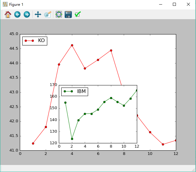
3.5 子图 axes:p1 = pl.axes([.1,.1,0.8,0.8]) # axes([left,bottom,width,height])(参数范围为(0,1))
参考:http://www.xuebuyuan.com/491377.html
p1 = pl.axes([.1,.1,0.8,0.8])  # axes([left,bottom,width,height])
p2 = pl.axes([.3,.15,0.4,0.4])

p1.plot(list1Index,list11,color='r',marker='o',label='KO')
p1.legend(loc='upper left')

p2.plot(list2Index,list22,color='g',marker='o',label='IBM')
p2.legend(loc='upper left')

pl.show()
4. Pandas作图
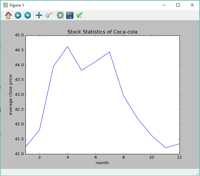
4.1 直接对Series进行绘图:closeMeansKO.plot() # KO公司12个月的月平均收盘价折线图
from matplotlib.finance import quotes_historical_yahoo_ochl
from datetime import date, datetime
import time
import pandas as pd
import matplotlib.pyplot as plt
today = date.today()
start = (today.year-1, today.month, today.day)
quotes = quotes_historical_yahoo_ochl('KO', start, today)
fields = ['date','open','close','high','low','volume']
list1 = []
for i in range(0,len(quotes)):
    x = date.fromordinal(int(quotes[i][0]))
    y = datetime.strftime(x,'%Y-%m-%d')
    list1.append(y)
#print(list1)
quoteskodf = pd.DataFrame(quotes, index = list1, columns = fields)
quoteskodf = quoteskodf.drop(['date'], axis = 1)
#print(quotesdf)
listtemp = []
for i in range(0,len(quoteskodf)):
    temp = time.strptime(quoteskodf.index[i],"%Y-%m-%d")  # 提取月份
    listtemp.append(temp.tm_mon)
#print(listtemp) # “print listtemp” in Python 2.x
tempkodf = quoteskodf.copy()
tempkodf['month'] = listtemp
closeMeansKO = tempkodf.groupby('month').mean().close

closeMeansKO.plot()
plt.title('Stock Statistics of Coca-cola')
plt.xlabel('month')
plt.ylabel('average close price')
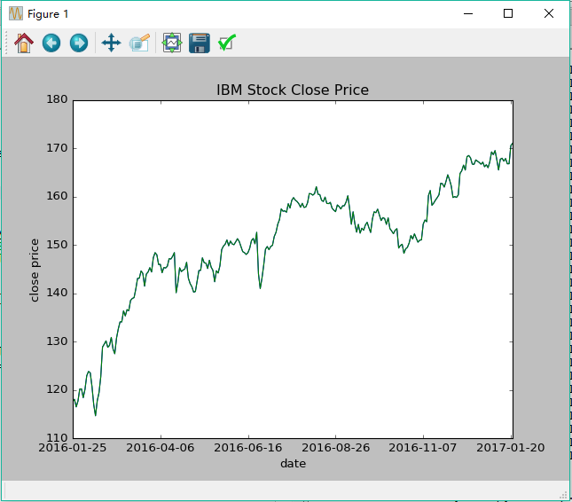
4.2 直接对DataFrame进行绘图:quotesdf.close.plot() # IBM公司近一年收盘价折线图
# -*- coding: utf-8 -*-
"""
Created on Tue Jan 24 13:07:01 2017

@author: Wayne
"""

from matplotlib.finance import quotes_historical_yahoo_ochl
from datetime import date, datetime
import pandas as pd
import matplotlib.pyplot as plt

today = date.today()
start = (today.year-1, today.month, today.day)
quotes = quotes_historical_yahoo_ochl('IBM', start, today)
fields = ['date','open','close','high','low','volume']
list1 = []
for i in range(0,len(quotes)):
    x = date.fromordinal(int(quotes[i][0]))
    y = datetime.strftime(x,'%Y-%m-%d')
    list1.append(y)
#print(list1)
quotesdf = pd.DataFrame(quotes, index = list1, columns = fields)
quotesdf = quotesdf.drop(['date'], axis = 1)

plt.title('IBM Stock Close Price')
plt.xlabel('date')
plt.ylabel('close price')
quotesdf.close.plot()
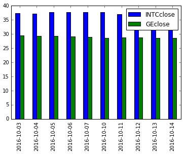
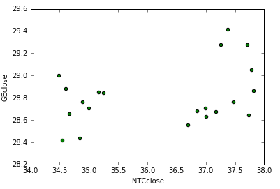
4.3 Pandas控制图像形式:quotesdf.plot(kind='bar')(用柱状图比较Intel和GE两家科技公司2014年10月的股票收盘价)
# -*- coding: utf-8 -*-
"""
Created on Tue Jan 24 13:07:01 2017

@author: Wayne
"""

from matplotlib.finance import quotes_historical_yahoo_ochl
from datetime import date, datetime
import pandas as pd

start = date(2016,10,01)
end = date(2016,10,16)
quotes1 = quotes_historical_yahoo_ochl('INTC', start, end)
quotes2 = quotes_historical_yahoo_ochl('GE', start, end)
fields = ['date','open','close','high','low','volume']
list1 = []
list2 = []
for i in range(0,len(quotes1)):
    x = date.fromordinal(int(quotes1[i][0]))
    y = datetime.strftime(x,'%Y-%m-%d')
    list1.append(y)
for i in range(0,len(quotes2)):
    x = date.fromordinal(int(quotes2[i][0]))
    y = datetime.strftime(x,'%Y-%m-%d')
    list2.append(y)

quotesdf1 = pd.DataFrame(quotes1, index = list1, columns = fields)
quotesdf1 = quotesdf1.drop(['date'], axis = 1)
quotesdf2 = pd.DataFrame(quotes2, index = list2, columns = fields)
quotesdf2 = quotesdf2.drop(['date'], axis = 1)

quotesdf = pd.DataFrame()
quotesdf['INTCclose'] = quotesdf1.close
quotesdf['GEclose'] = quotesdf2.close
quotesdf.plot(kind='bar')
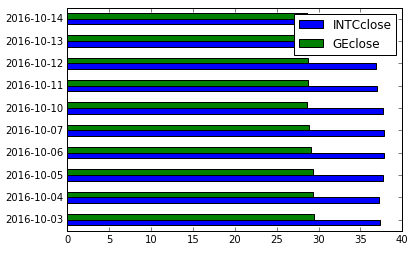
[ quotesdf.plot(kind='bar') ] [ quotesdf.plot(kind='barh') ] [ quotesdf.plot(kind='scatter', x='INTCclose', y='GEclose', color='g') ]
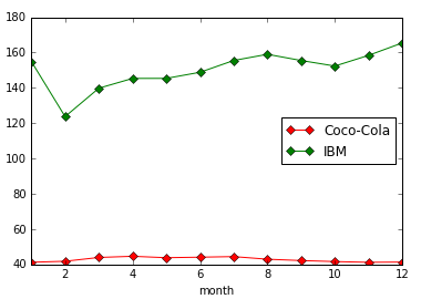
4.4 Pandas控制图像属性:将KO公司和IBM公司近12个月收盘平均价绘制在同一张图上
closeMeans1.plot(color='r',marker='D',label='Coco-Cola')
closeMeans2.plot(color='g',marker='D',label='IBM')
plt.legend(loc='center right')
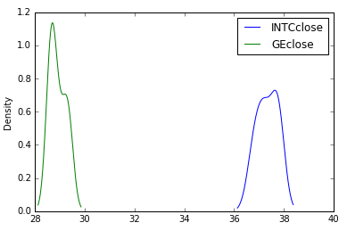
4.5 Pandas控制图像属性:绘图显示Intel和GE两家科技公司2014年10月的股票收盘价的概率分布
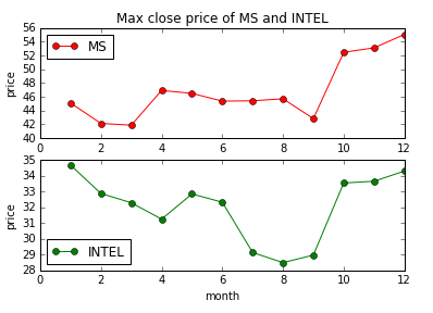
4.6 练习:用折线图比较Microsoft 和Intel 在2015 年每个月股票的最高收盘价。图标题为“MaxClose of MS and INTEL”,横坐标是时间,纵坐标是价格
# -*- coding: utf-8 -*-
"""
Created on Tue Jan 24 13:07:01 2017

@author: Wayne
"""

from matplotlib.finance import quotes_historical_yahoo_ochl
from datetime import date, datetime
import time
import pandas as pd
import matplotlib.pylab as pl

start = date(2015,01,01)
end = date(2016,01,01)

quotes1 = quotes_historical_yahoo_ochl('MSFT', start, end)
quotes2 = quotes_historical_yahoo_ochl('INTC', start, end)
fields = ['date','open','close','high','low','volume']
list1 = []
list2 = []
for i in range(0,len(quotes1)):
    x = date.fromordinal(int(quotes1[i][0]))
    y = datetime.strftime(x,'%Y-%m-%d')
    list1.append(y)
for i in range(0,len(quotes2)):
    x = date.fromordinal(int(quotes2[i][0]))
    y = datetime.strftime(x,'%Y-%m-%d')
    list2.append(y)

quoteskodf1 = pd.DataFrame(quotes1, index = list1, columns = fields)
quoteskodf1 = quoteskodf1.drop(['date'], axis = 1)
quoteskodf2 = pd.DataFrame(quotes2, index = list2, columns = fields)
quoteskodf2 = quoteskodf2.drop(['date'], axis = 1)

listtemp1 = []
listtemp2 = []
for i in range(0,len(quoteskodf1)):
    temp = time.strptime(quoteskodf1.index[i],"%Y-%m-%d")  # 提取月份
    listtemp1.append(temp.tm_mon)
for i in range(0,len(quoteskodf2)):
    temp = time.strptime(quoteskodf2.index[i],"%Y-%m-%d")  # 提取月份
    listtemp2.append(temp.tm_mon)

tempdf1 = quoteskodf1.copy()
tempdf1['month'] = listtemp1
closeMeans1 = tempdf1.groupby('month').max().close
list11 = []
for i in range(1,13):
    list11.append(closeMeans1[i])
list1Index = closeMeans1.index

tempdf2 = quoteskodf2.copy()
tempdf2['month'] = listtemp2
closeMeans2 = tempdf2.groupby('month').max().close
list22 = []
for i in range(1,13):
    list22.append(closeMeans2[i])
list2Index = closeMeans2.index

p1 = pl.subplot(211)
p2 = pl.subplot(212)

p1.set_title('Max close price of MS and INTEL')
p1.plot(list1Index,list11,color='r',marker='o',label='MS')
p1.set_ylabel('price')
p1.legend(loc='upper left')

p2.plot(list2Index,list22,color='g',marker='o',label='INTEL')
p2.set_xlabel('month')
p2.set_ylabel('price')
p2.legend(loc='lower left')

pl.show()