Likelihood principle【转】

Likelihood principle

From Wikipedia, the free encyclopedia

In statistics, the likelihood principle is a controversial principle of statistical inference which asserts that all of the information in a sample is contained in thelikelihood function.

A likelihood function arises from a conditional probability distribution considered as a function of its distributional parameterization argument, conditioned on the data argument.

For example, consider a model which gives the probability density function of observable random variable X as a function of a parameter θ. Then for a specific valuex of X,

the function L(θ | x) = P(X=x | θ) is a likelihood function of θ: it gives a measure of how "likely" any particular value of θ is, if we know that X has the valuex.

Two likelihood functions are equivalent if one is a scalar multiple of the other. The likelihood principle states that all information from the data relevant to inferences about

the value of θ is found in the equivalence class. The strong likelihood principle applies this same criterion to cases such as sequential experiments where the sample of data

that is available results from applying a stopping rule to the observations earlier in the experiment.^[1]

[hide]

[edit]Example

Suppose

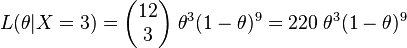
X is the number of successes in twelve independent Bernoulli trials with probability θ of success on each trial, and
Y is the number of independent Bernoulli trials needed to get three successes, again with probability θ of success on each trial.

Then the observation that X = 3 induces the likelihood function

$L(\theta|X=3)=\begin{pmatrix}12\\3\end{pmatrix}\;\theta^3(1-\theta)^9=220\;\theta^3(1-\theta)^9$

and the observation that Y = 12 induces the likelihood function

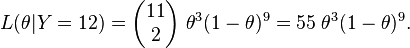
$L(\theta|Y=12)=\begin{pmatrix}11\\2\end{pmatrix}\;\theta^3(1-\theta)^9=55\;\theta^3(1-\theta)^9.$

These are equivalent because each is a scalar multiple of the other. The likelihood principle therefore says the inferences drawn about the value of θ should be the same in

both cases.

The difference between observing X = 3 and observing Y = 12 is only in the design of the experiment: in one case, one has decided in advance to try twelve times;

in the other, to keep trying until three successes are observed. The outcome is the same in both cases.

[edit]The law of likelihood

A related concept is the law of likelihood, the notion that the extent to which the evidence supports one parameter value or hypothesis against another is equal to the

ratio of their likelihoods. That is,

$\Lambda = {L(a|X=x) \over L(b|X=x)} = {P(X=x|a) \over P(X=x|b)}$

is the degree to which the observation x supports parameter value or hypothesis a against b. If this ratio is 1, the evidence is indifferent, and if greater or less than 1,

the evidence supports a against b or vice versa. The use of Bayes factors can extend this by taking account of the complexity of different hypotheses.

Combining the likelihood principle with the law of likelihood yields the consequence that the parameter value which maximizes the likelihood function is the value which

is most strongly supported by the evidence. This is the basis for the widely-used method of maximum likelihood.

[edit]Historical remarks

The likelihood principle was first identified by that name in print in 1962 (Barnard et al., Birnbaum, and Savage et al.), but arguments for the same principle, unnamed,

and the use of the principle in applications goes back to the works of R.A. Fisher in the 1920s. The law of likelihood was identified by that name by I. Hacking (1965).

More recently the likelihood principle as a general principle of inference has been championed by A. W. F. Edwards. The likelihood principle has been applied to the

philosophy of science by R. Royall.Birnbaum proved that the likelihood principle follows from two more primitive and seemingly reasonable principles, the conditionality

principle and the sufficiency principle. The conditionality principle says that if an experiment is chosen by a random process independent of the states of nature $θ$ , then only

the experiment actually performed is relevant to inferences about $θ$ . The sufficiency principle says that if $T (X)$ is a sufficient statistic for $θ$ , and if in two experiments with

data $x 1$ and $x 2$ we have $T (x 1) = T (x 2)$ , then the evidence about $θ$ given by the two experiments is the same.

[edit]Arguments for and against the likelihood principle

The likelihood principle is not universally accepted. Some widely-used methods of conventional statistics, for example many significance tests, are not consistent with the

likelihood principle. Let us briefly consider some of the arguments for and against the likelihood principle.

[edit]Experimental design arguments on the likelihood principle

Unrealized events do play a role in some common statistical methods. For example, the result of a significance test depends on the probability of a result as extreme or

more extreme than the observation, and that probability may depend on the design of the experiment. Thus, to the extent that such methods are accepted, the likelihood

principle is denied.

Some classical significance tests are not based on the likelihood. A commonly cited example is the optional stopping problem. Suppose I tell you that I tossed a coin 12 times

and in the process observed 3 heads. You might make some inference about the probability of heads and whether the coin was fair. Suppose now I tell that I tossed the coin

until I observed 3 heads, and I tossed it 12 times. Will you now make some different inference?

The likelihood function is the same in both cases: it is proportional to

$p^3 \; (1-p)^9$ .

According to the likelihood principle, the inference should be the same in either case.

Suppose a number of scientists are assessing the probability of a certain outcome (which we shall call 'success') in experimental trials. Conventional wisdom suggests that if there

is no bias towards success or failure then the success probability would be one half. Adam, a scientist, conducted 12 trials and obtains 3 successes and 9 failures. Then he left the lab.

Bill, a colleague in the same lab, continued Adam's work and published Adam's results, along with a significance test. He tested the null hypothesis that p, the success probability,

is equal to a half, versus p < 0.5. The probability of the observed result that out of 12 trials 3 or something fewer (i.e. more extreme) were successes, if H₀ is true, is

$\left({12 \choose 9}+{12 \choose 10}+{12 \choose 11}+{12 \choose 12}\right)\left({1 \over 2}\right)^{12}$

which is 299/4096 = 7.3%. Thus the null hypothesis is not rejected at the 5% significance level.

Charlotte, another scientist, reads Bill's paper and writes a letter, saying that it is possible that Adam kept trying until he obtained 3 successes, in which case the probability of needing to

conduct 12 or more experiments is given by

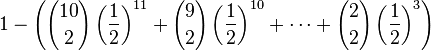
$1-\left({10 \choose 2}\left({1 \over 2}\right)^{11}+{9 \choose 2}\left({1 \over 2}\right)^{10}+\cdots +{2 \choose 2}\left({1 \over 2}\right)^{3}\right)$

which is 134/4096 = 3.27%. Now the result is statistically significant at the 5% level.

To these scientists, whether a result is significant or not seems to depend on the original design of the experiment, not just the likelihood of the outcome.

Paradoxical results of this kind are considered by some as arguments against the likelihood principle. For others it exemplifies the value of the likelihood principle and is an argument against

significance tests which, for them, resolves the paradox.

It is worth noting that there is no real contradiction in this example. Bill's result is the probability of obtaining 3 or fewer successes in 12 trials. Charlotte's result is the probability that the 3rd

success will occur on the 12th or later trial. These are fundamentally different things. The probability of obtaining 3 or fewer successes in 12 trials properly maps to the probability that the 4th

success occurs after the 12th trial. By taking only the cases in which the 3rd success occurs on the 12th trial or later, those cases are ignored in which the 3rd success happens earlier and is

followed by a string of failures up to the 12th trial; this accounts for the difference in the calculations. Another way of looking at this is that Charlotte's calculation implicitly assumes that the

3rd success occurs on the 12th trial, something that is not clear in the problem statement and that is not assumed in Bill's calculation. From Bill's perspective, Charlotte's calculation is the same

as the probability of obtaining 2 or fewer successes in 11 trials, given a success on the 12th trial.

Similar themes appear when comparing Fisher's exact test with Pearson's chi-squared test.

[edit]The voltmeter story

An argument in favor of the likelihood principle is given by Edwards in his book Likelihood. He cites the following story from J.W. Pratt, slightly condensed here. Note that the likelihood function

depends only on what actually happened, and not on what could have happened.

An engineer draws a random sample of electron tubes and measures their voltage. The measurements range from 75 to 99 volts. A statistician computes the sample mean and a confidence

interval for the true mean. Later the statistician discovers that the voltmeter reads only as far as 100, so the population appears to be 'censored'. This necessitates a new analysis, if the

statistician is orthodox. However, the engineer says he has another meter reading to 1000 volts, which he would have used if any voltage had been over 100. This is a relief to the statistician,

because it means the population was effectively uncensored after all. But, the next day the engineer informs the statistician that this second meter was not working at the time of the measuring.

The statistician ascertains that the engineer would not have held up the measurements until the meter was fixed, and informs him that new measurements are required. The engineer is astounded.

"Next you'll be asking about my oscilloscope".

One might proceed with this story, and consider the fact that in general the actual situation could have been different. For instance, high range voltmeters don't break at predictable moments in time,

but rather at unpredictable moments. So it could have been broken, with some probability. The likelihood theory claims that the distribution of the voltage measurements depends on the probability

that an instrument not used in this experiment was broken at the time.

This story can be translated to Adam's stopping rule above, as follows. Adam stopped immediately after 3 successes, because his boss Bill had instructed him to do so. Adam did not die. After the

publication of the statistical analysis by Bill, Adam discovers that he has missed a second instruction from Bill to conduct 12 trials instead, and that Bill's paper is based on this second instruction.

Adam is very glad that he got his 3 successes after exactly 12 trials, and explains to his friend Charlotte that by coincidence he executed the second instruction. Later, he is astonished to hear

about Charlotte's letter explaining that now the result is significant.

[edit]Optional stopping in clinical trials

This section does not cite any references or sources. Please help improve this section by adding citations to reliable sources. Unsourced material may be challenged and removed. (October 2011)

The fact that Bayesian and frequentist arguments differ on the subject of optional stopping has a major impact on the way that clinical trial data can be analysed. In frequentist setting there is a major

difference between a design which is fixed and one which is sequential, i.e. consisting of a sequence of analyses. Bayesian statistics is inherently sequential and so there is no such distinction.

In a clinical trial it is strictly not valid to conduct an unplanned interim analysis of the data by frequentist methods, whereas this is permissible by Bayesian methods. Similarly, if funding is withdrawn

part way through an experiment, and the analyst must work with incomplete data, this is a possible source of bias for classical methods but not for Bayesian methods, which do not depend on the

intended design of the experiment. Furthermore, as mentioned above, frequentist analysis is open to unscrupulous manipulation if the experimenter is allowed to choose the stopping point, whereas

Bayesian methods are immune to such manipulation.

[edit]See also

[edit]References

^ Dodge, Y. (2003) The Oxford Dictionary of Statistical Terms. OUP. ISBN 0-19-920613-9

Barnard, G.A.; G.M. Jenkins, and C.B. Winsten (1962). "Likelihood Inference and Time Series". J. Royal Statistical Society, A 125 (3): 321–372. doi:10.2307/2982406.ISSN 0035-9238. JSTOR 2982406.
Berger, J.O.; and Wolpert, R.L. (1988). The Likelihood Principle (2nd ed.). Haywood, CA: The Institute of Mathematical Statistics. ISBN 0-940600-13-7.
Birnbaum, Allan (1962). "On the foundations of statistical inference". J. Amer. Statist. Assoc. 57 (298): 269–326. doi:10.2307/2281640. ISSN 0162-1459. JSTOR 2281640.MR 0138176. (With discussion.)
Edwards, Anthony W.F. (1972). Likelihood (1st ed.). Cambridge: Cambridge University Press.
Edwards, Anthony W.F. (1992). Likelihood (2nd ed.). Baltimore: Johns Hopkins University Press. ISBN 0-8018-4445-2.
Edwards, Anthony W.F. (1974). "The history of likelihood". International Statistical Review 42 (1): 9–15. doi:10.2307/1402681. ISSN 0306-7734. JSTOR 1402681.MR 0353514.
Fisher, Ronald A. (1922). "On the Mathematical Foundations of Theoretical Statistics" (PDF fulltext). Phil. Trans. Royal Soc. A 222 (594–604): 326.doi:10.1098/rsta.1922.0009. Retrieved 2008-12-28.
Hacking, Ian (1965). Logic of Statistical Inference. Cambridge: Cambridge University Press. ISBN 0-521-05165-7.
Jeffreys, Harold (1961). The Theory of Probability. The Oxford University Press.
Royall, Richard M. (1997). Statistical Evidence: A Likelihood Paradigm. London: Chapman & Hall. ISBN 0-412-04411-0.
Savage, Leonard J.; et al. (1962). The Foundations of Statistical Inference. London: Methuen.

[edit]External links

Anthony W.F. Edwards. "Likelihood". http://www.cimat.mx/reportes/enlinea/D-99-10.html
Jeff Miller. Earliest Known Uses of Some of the Words of Mathematics (L)
John Aldrich. Likelihood and Probability in R. A. Fisher’s Statistical Methods for Research Workers

转自：http://en.wikipedia.org/wiki/Likelihood_principle