吴裕雄--天生自然 R语言开发学习：时间序列

#-----------------------------------------#
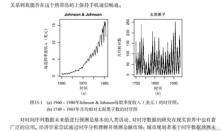
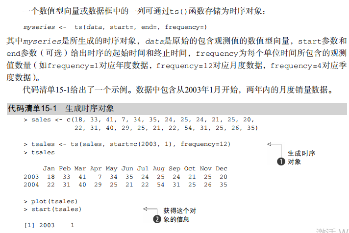
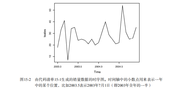
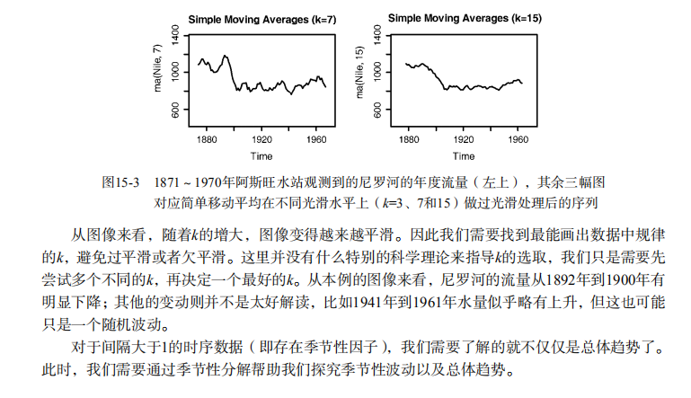
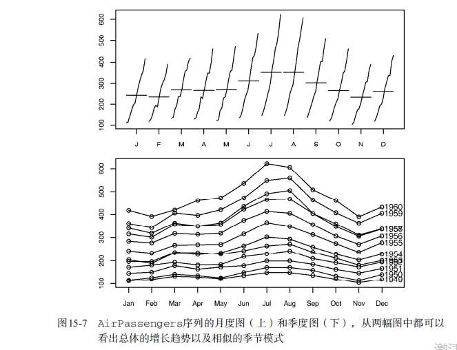
# R in Action (2nd ed): Chapter 15        #
# Time series                             #
# requires forecast, tseries packages     #
# install.packages("forecast", "tseries") #
#-----------------------------------------#

par(ask=TRUE)

# Listing 15.1 - Creating a time series object in R
sales <- c(18, 33, 41,  7, 34, 35, 24, 25, 24, 21, 25, 20, 
           22, 31, 40, 29, 25, 21, 22, 54, 31, 25, 26, 35)
tsales <- ts(sales, start=c(2003, 1), frequency=12) 
tsales
plot(tsales)

start(tsales) 
end(tsales)
frequency(tsales)

tsales.subset <- window(tsales, start=c(2003, 5), end=c(2004, 6))
tsales.subset


# Listing 15.2 - Simple moving averages
library(forecast)
opar <- par(no.readonly=TRUE)
par(mfrow=c(2,2))
ylim <- c(min(Nile), max(Nile))
plot(Nile, main="Raw time series")
plot(ma(Nile, 3), main="Simple Moving Averages (k=3)", ylim=ylim)
plot(ma(Nile, 7), main="Simple Moving Averages (k=7)", ylim=ylim)
plot(ma(Nile, 15), main="Simple Moving Averages (k=15)", ylim=ylim)
par(opar)


# Listing 15.3 - Seasonal decomposition using slt()
plot(AirPassengers)                                               
lAirPassengers <- log(AirPassengers)
plot(lAirPassengers, ylab="log(AirPassengers)")
fit <- stl(lAirPassengers, s.window="period")           
plot(fit)
fit$time.series                                 
exp(fit$time.series)


par(mfrow=c(2,1))
library(forecast)
monthplot(AirPassengers, xlab="",  ylab="")  
seasonplot(AirPassengers, year.labels="TRUE", main="")
par(opar)


# Listing 15.4 - Simple exponential smoothing
library(forecast) 
fit <- HoltWinters(nhtemp, beta=FALSE, gamma=FALSE)      
fit

forecast(fit, 1)  

plot(forecast(fit, 1), xlab="Year", 
     ylab=expression(paste("Temperature (", degree*F,")",)),
     main="New Haven Annual Mean Temperature") 

accuracy(fit)                                            


# Listing 15.5 - Exponential smoothing with level, slope, and seasonal components
fit <- HoltWinters(log(AirPassengers))      
fit

accuracy(fit)

pred <- forecast(fit, 5)                                  
pred
plot(pred, main="Forecast for Air Travel", 
     ylab="Log(AirPassengers)", xlab="Time")       
pred$mean <- exp(pred$mean)
pred$lower <- exp(pred$lower)
pred$upper <- exp(pred$upper)
p <- cbind(pred$mean, pred$lower, pred$upper)
dimnames(p)[[2]] <- c("mean", "Lo 80", "Lo 95", "Hi 80", "Hi 95")
p


# Listing 15.6 - Automatic exponential forecasting with ets()
library(forecast)
fit <- ets(JohnsonJohnson)
fit
plot(forecast(fit), main="Johnson and Johnson Forecasts", 
     ylab="Quarterly Earnings (Dollars)", xlab="Time")


# Listing 15.7 - Transforming the time series and assessing stationarity
library(forecast)
library(tseries)
plot(Nile)
ndiffs(Nile)
dNile <- diff(Nile)                                              
plot(dNile)
adf.test(dNile)


# Listing 15.8 - Fit an ARIMA model
fit <- arima(Nile, order=c(0,1,1))                                 
fit
accuracy(fit)


# Listing 15.9 - Evaluating the model fit
qqnorm(fit$residuals)     
qqline(fit$residuals)
Box.test(fit$residuals, type="Ljung-Box")


# Listing 15.10 - Forecasting with an ARIMA model
forecast(fit, 3)
plot(forecast(fit, 3), xlab="Year", ylab="Annual Flow")


# Listing 15.11 - Automated ARIMA forecasting
library(forecast)
fit <- auto.arima(sunspots)
fit
forecast(fit, 3)
accuracy(fit)