原文链接:http://tecdat.cn/?p=18927
本文使用波兰公寓价格数据说明Fisher检验。
-
-
with(data = apart , boxplot(price ~ dis ))
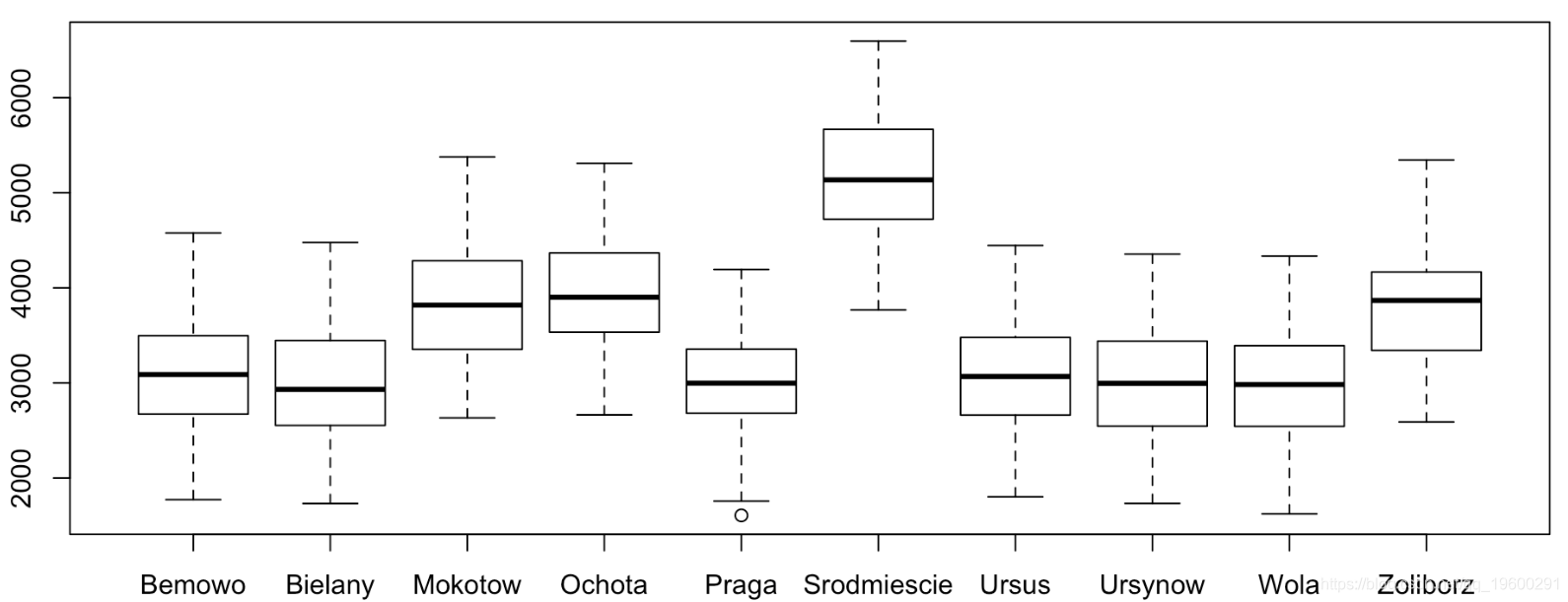
我们在这里对公寓进行分组(这也可以通过简单的回归,这里5个解释变量并不重要)。我们可以重新排列
A = A[order(A$x),]
我们以这里最便宜的地区为参考,
-
-
-
Coefficients:
-
Estimate Std. Error t value Pr(>|t|)
-
(Intercept) 2968.36 58.02 51.160 <2e-16 ***
-
districtBielany 17.38 84.16 0.207 0.836
-
districtPraga 26.45 85.12 0.311 0.756
-
districtUrsynow 42.01 82.65 0.508 0.611
-
districtBemowo 80.10 83.71 0.957 0.339
-
districtUrsus 102.01 82.25 1.240 0.215
-
districtZoliborz 829.59 83.94 9.884 <2e-16 ***
-
districtMokotow 887.10 81.86 10.837 <2e-16 ***
-
districtOchota 987.93 84.16 11.738 <2e-16 ***
-
districtSrodmiescie 2214.39 83.28 26.591 <2e-16 ***
-
-
Signif. codes: 0 ‘***’ 0.001 ‘**’ 0.01 ‘*’ 0.05 ‘.’ 0.1 ‘ ’ 1
-
-
Residual standard error: 597.4 on 990 degrees of freedom
-
Multiple R-squared: 0.5698, Adjusted R-squared: 0.5659
-
F-statistic: 145.7 on 9 and 990 DF, p-value: < 2.2e-16
我们可以检验前5个地区价格,这是一个多重检验,我们将使用Fisher检验:
-
-
linHypo(reg, c("districtBielany = 0"
-
"districtPraga = 0"
-
"districtUrsynow = 0"
-
"districtBemowo = 0"
-
"districtUrsus = 0")
-
Linear hypothesis test
-
-
Model 1: restricted model
-
Model 2: m2.price ~ district
-
-
Res.Df RSS Df Sum of Sq F Pr(>F)
-
1 995 354051715
-
2 990 353269202 5 782513 0.4386 0.8217
Fisher的统计数据很低, p值为82%。
-
-
Linear hypothesis test
-
-
Model 1: restricted model
-
Model 2: m2.price ~ district
-
-
Res.Df RSS Df Sum of Sq F Pr(>F)
-
1 996 405455409
-
2 990 353269202 6 52186207 24.374 < 2.2e-16 ***
-
-
Signif. codes: 0 ‘***’ 0.001 ‘**’ 0.01 ‘*’ 0.05 ‘.’ 0.1 ‘ ’ 1
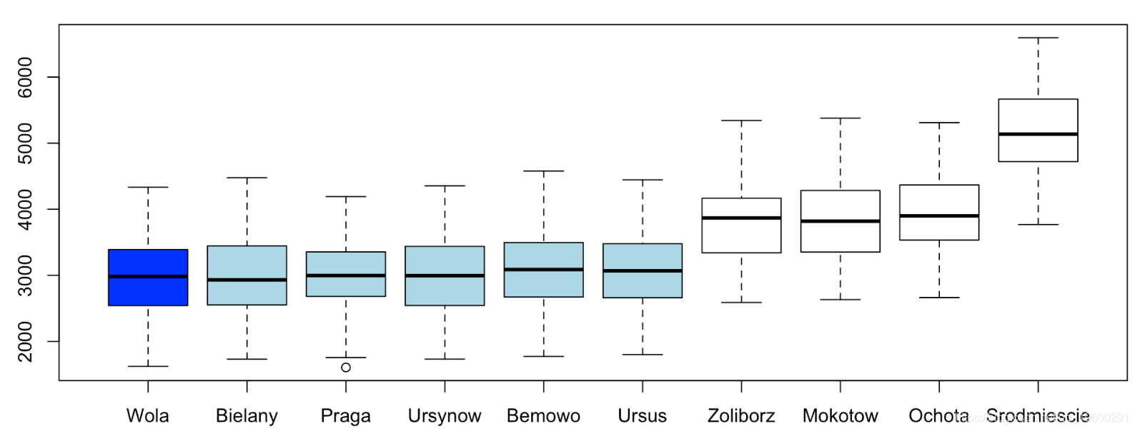
我们将对前6种地区进行重组(并称A为地区重组)。如果我们看平均价格,按地区,我们得到
with(data = apar , boxplot( price ~ distr ))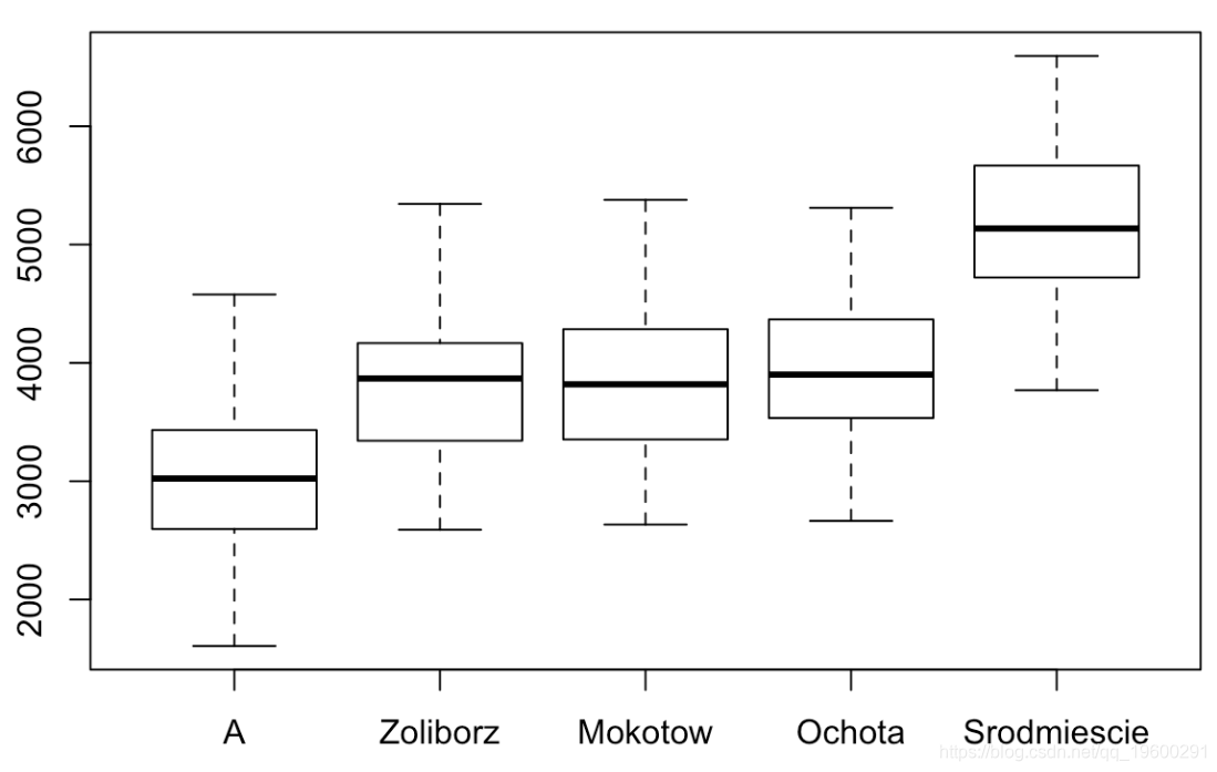
我们再次开始,以最便宜的地区作为参考,我们想检验线性回归中接下来的两个地区的系数是否为零。
-
-
Linear hypothesis test
-
-
Model 1: restricted model
-
Model 2: m2.price ~ district
-
-
Res.Df RSS Df Sum of Sq F Pr(<F)
-
1 997 355292524
-
2 995 354051715 2 1240809 1.7435 0.1754
P为0.17,我们可以接受原假设。然后,我们有三组地区,名称分别为A,B和C。我们获得以下框线图
-
-
with(data = apart , boxplot( price ~ dist ))
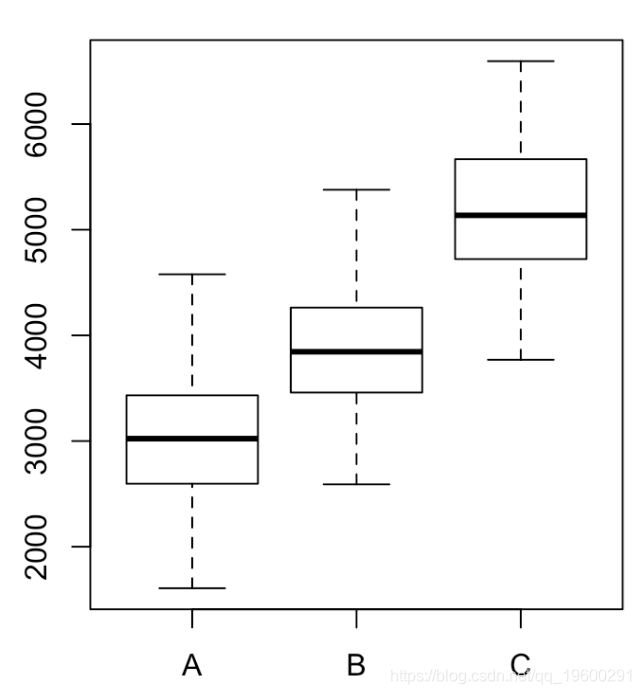
因此,最终我们可以分类成三个不同的地区,如果目标是预测价格,则无需使用10类分类,而3类分类就足够了!

最受欢迎的见解
1.Matlab马尔可夫链蒙特卡罗法(MCMC)估计随机波动率(SV,Stochastic Volatility) 模型
3.WinBUGS对多元随机波动率模型:贝叶斯估计与模型比较
4.R语言回归中的hosmer-lemeshow拟合优度检验