建立ARMAX模型需要运用R的dse包,在R的dse包中The ARMA model representation is general, so that VAR, VARX,ARIMA, ARMAX, ARIMAX can all be considered to be special cases.
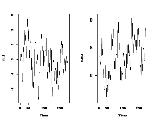
数据集为天然气炉中的天然气(input)与产生的CO2(output),数据来源为王燕应用时间序列分析第三版附录表A1-24,首先队数据做简要的分析,做出时序图以及协方差图
input<-ts(input,frequency = 1,start = c(1,1))

output<-ts(output,frequency = 1,start = c(1,1))

par(mfrow=c(1,2))

plot.ts(input)

plot.ts(output)
做两个变量间的协方差函数需要使用ccf函数
ccf(output,input,lag.max = NULL,type = c("correlation"),plot = TRUE)

可以看到两变量存在逻辑上的因果关系,变量延迟的阶数在3~5左右,因此可以通过dse包进行建模,需要使用的函数有ARMA,TSdata,estMaxLik,forecast
首先使用ARMA函数定义一个模型表达式,注意ARMA只能定义一个模型结构,而不能估计其参数,其定义的结构为
A(L)y(t) = B(L)w(t) + C(L)u(t) + TREND(t)
where
A (axpxp) is the auto-regressive polynomial array.
B (bxpxp) is the moving-average polynomial array.
C (cxpxm) is the input polynomial array. C should be NULL if there is no input
y is the p dimensional output data.
u is the m dimensional control (input) data.
TREND is a matrix the same dimension as y, a p-vector (which gets replicated for each time
period), or NULL.
需要注意定义模型中参数与变量的区别,以及模型设置的初始值设置
By default, elements in parameter arrays are treated as constants if they are exactly 1.0 or 0.0, and
as parameters otherwise. A value of 1.001 would be treated as a parameter, and this is the easiest
way to initialize an element which is not to be treated as a constant of value 1.0. Any array elements
can be fixed to constants by specifying the list constants. Arrays which are not specified in the list
will be treated in the default way. An alternative for fixing constants is the function fixConstants.
因此我们可以如下定义模型
MA <- array(c(1,-1.5,0.5),c(3,1,1))

C <- array(c(0,0,0,-0.5,-0.5,-0.5),c(5,1,1))

AR <- array(c(1,-0.5),c(2,1,1))

TR <-array(c(50),c(1,1,1))

ARMAX <- ARMA(A=AR, B=MA, C=C ,TREND<-TR)
定义好模型后,还需要将数据转化为需要的格式,这里要使用TSdata函数,把input与output数据存储在一起
随后就可以使用estMaxLik函数对模型进行求解了,先说另一个求解函数estVARXls,顾名思义,采用的求解方法为ls,该函数的好处是可以自动定阶,如:
armaxdata<-TSdata(input=input,output=output)

model <- estVARXls(armaxdata)
> model
neg. log likelihood= 821.601
A(L) =
1-1.705922L1+0.6411281L2+0.2290077L3-0.128453L4-0.0686206L5+0.03279703L6
B(L) =
1
C(L) =
-0.08792481+0.2803458L1-0.2801545L2-0.3750078L3-0.07263863L4+0.5139702L5
如果想要用前面设置的ARMA形式来建模的话则需要使用estMaxLik,该函数采用Maximum likelihood estimation,注意每次计算的结果可能与ARMA设置的初始值有关,如果想要得到更好的结果,需要对该函数参数进行讨论。
model <- estMaxLik(armaxdata, ARMAX, algorithm="optim")
> model
neg. log likelihood= 231.8164
TREND= 53.493
A(L) =
1+0.001700993L1
B(L) =
1+1.486967L1+0.7612954L2
C(L) =
0-1.002061L3-1.601826L4
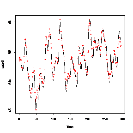
最后还要使用forecast函数对模型进行预测,注意如果input和output一样长,则不会产生新的未来预测值,但是会产生模型拟合值pred,如果想要对未来进行预测,需要讨论conditioning.inputs.forecasts(A time series matrix or list of time series matrices to append to input variables for the forecast periods.)
pr <- forecast(model, conditioning.inputs=inputData(armaxdata))
提取出pred项画出预测图
pred<-ts(as.vector(pr$pred),frequency = 1,start = c(1,1))
plot(pred,col="red",type="p")
par(new=TRUE)
plot(output)
笔者也是ARMAX初学者,若有错误请大家指出