PCA

http://deeplearning.stanford.edu/wiki/index.php/PCA

Principal Components Analysis (PCA) is a dimensionality reduction algorithm that can be used to significantly speed up your unsupervised feature learning algorithm.

example

Suppose you are training your algorithm on images. Then the input will be somewhat redundant, because the values of adjacent pixels in an image are highly correlated. Concretely, suppose we are training on 16x16 grayscale image patches. Then $extstyle x in Re^{256}$ are 256 dimensional vectors, with one feature $extstyle x_j$ corresponding to the intensity of each pixel. Because of the correlation between adjacent pixels, PCA will allow us to approximate the input with a much lower dimensional one, while incurring very little error.

PCA will find a lower-dimensional subspace onto which to project our data. From visually examining the data, it appears that $extstyle u_1$ is the principal direction of variation of the data, and $extstyle u_2$ the secondary direction of variation:

the data varies much more in the direction $extstyle u_1$ than $extstyle u_2$ .

To more formally find the directions $extstyle u_1$ and $extstyle u_2$ , we first compute the matrix $extstyle Sigma$ as follows:

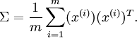
$egin{align} Sigma = frac{1}{m} sum_{i=1}^m (x^{(i)})(x^{(i)})^T. end{align}$

If $extstyle x$ has zero mean, then $extstyle Sigma$ is exactly the covariance matrix of $extstyle x$ . (The symbol " $extstyle Sigma$ ", pronounced "Sigma", is the standard notation for denoting the covariance matrix. Unfortunately it looks just like the summation symbol, as in $sum_{i=1}^n i$ ; but these are two different things.)

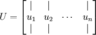
let us compute the eigenvectors of $extstyle Sigma$ , and stack the eigenvectors in columns to form the matrix $extstyle U$ :

$egin{align} U = egin{bmatrix} | & | & & | \ u_1 & u_2 & cdots & u_n \ | & | & & | end{bmatrix} end{align}$

Here, $extstyle u_1$ is the principal eigenvector (corresponding to the largest eigenvalue), $extstyle u_2$ is the second eigenvector, and so on. Also, let 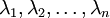$extstyle lambda_1, lambda_2, ldots, lambda_n$ be the corresponding eigenvalues.

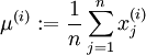
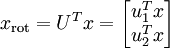
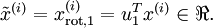
The vectors $extstyle u_1$ and $extstyle u_2$ in our example form a new basis in which we can represent the data. Concretely, let $extstyle x in Re^2$ be some training example. Then $extstyle u_1^Tx$ is the length (magnitude) of the projection of $extstyle x$ onto the vector $extstyle u_1$ .

Similarly, $extstyle u_2^Tx$ is the magnitude of $extstyle x$ projected onto the vector $extstyle u_2$ .

Rotating the Data

Thus, we can represent $extstyle x$ in the $extstyle (u_1, u_2)$ -basis by computing

$egin{align} x_{ m rot} = U^Tx = egin{bmatrix} u_1^Tx \ u_2^Tx end{bmatrix} end{align}$

(The subscript "rot" comes from the observation that this corresponds to a rotation (and possibly reflection) of the original data.) Lets take the entire training set, and compute $extstyle x_{ m rot}^{(i)} = U^Tx^{(i)}$ for every $extstyle i$ . Plotting this transformed data $extstyle x_{ m rot}$ , we get:

This is the training set rotated into the $extstyle u_1$ , $extstyle u_2$ basis. In the general case, $extstyle U^Tx$ will be the training set rotated into the basis $extstyle u_1$ , $extstyle u_2$ , ..., $extstyle u_n$ .

One of the properties of $extstyle U$ is that it is an "orthogonal" matrix, which means that it satisfies $extstyle U^TU = UU^T = I$ . So if you ever need to go from the rotated vectors $extstyle x_{ m rot}$ back to the original data $extstyle x$ , you can compute

$egin{align} x = U x_{ m rot} , end{align}$

because $extstyle U x_{ m rot} = UU^T x = x$ .

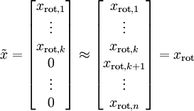
Reducing the Data Dimension

We see that the principal direction of variation of the data is the first dimension $extstyle x_{{ m rot},1}$ of this rotated data. Thus, if we want to reduce this data to one dimension, we can set

$egin{align} ilde{x}^{(i)} = x_{{ m rot},1}^{(i)} = u_1^Tx^{(i)} in Re. end{align}$

More generally, if $extstyle x in Re^n$ and we want to reduce it to a $extstyle k$ dimensional representation $extstyle ilde{x} in Re^k$ (where $extstyle k < n$ ), we would take the first $extstyle k$ components of $extstyle x_{ m rot}$ , which correspond to the top $extstyle k$ directions of variation.

$egin{align} ilde{x} = egin{bmatrix} x_{{ m rot},1} \ vdots \ x_{{ m rot},k} \ 0 \ vdots \ 0 \ end{bmatrix} approx egin{bmatrix} x_{{ m rot},1} \ vdots \ x_{{ m rot},k} \ x_{{ m rot},k+1} \ vdots \ x_{{ m rot},n} end{bmatrix} = x_{ m rot} end{align}$

In our example, this gives us the following plot of $extstyle ilde{x}$ (using $extstyle n=2, k=1$ ):

However, since the final $extstyle n-k$ components of $extstyle ilde{x}$ as defined above would always be zero, there is no need to keep these zeros around, and so we define $extstyle ilde{x}$ as a $extstyle k$ -dimensional vector with just the first $extstyle k$ (non-zero) components.

This also explains why we wanted to express our data in the $extstyle u_1, u_2, ldots, u_n$ basis: Deciding which components to keep becomes just keeping the top $extstyle k$ components. When we do this, we also say that we are "retaining the top $extstyle k$ PCA (or principal) components."

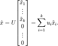
Recovering an Approximation of the Data

we can think of $extstyle ilde{x}$ as an approximation to $extstyle x_{ m rot}$ , where we have set the last $extstyle n-k$ components to zeros. Thus, given $extstyle ilde{x} in Re^k$ , we can pad it out with $extstyle n-k$ zeros to get our approximation to $extstyle x_{ m rot} in Re^n$ . Finally, we pre-multiply by $extstyle U$ to get our approximation to $extstyle x$ . Concretely, we get

$egin{align} hat{x} = U egin{bmatrix} ilde{x}_1 \ vdots \ ilde{x}_k \ 0 \ vdots \ 0 end{bmatrix} = sum_{i=1}^k u_i ilde{x}_i. end{align}$

We are thus using a 1 dimensional approximation to the original dataset.

Number of components to retain

To decide how to set $extstyle k$ , we will usually look at the percentage of variance retained for different values of $extstyle k$ . Concretely, if $extstyle k=n$ , then we have an exact approximation to the data, and we say that 100% of the variance is retained. I.e., all of the variation of the original data is retained. Conversely, if $extstyle k=0$ , then we are approximating all the data with the zero vector, and thus 0% of the variance is retained.

More generally, let $extstyle lambda_1, lambda_2, ldots, lambda_n$ be the eigenvalues of $extstyle Sigma$ (sorted in decreasing order), so that $extstyle lambda_j$ is the eigenvalue corresponding to the eigenvector $extstyle u_j$ . Then if we retain $extstyle k$ principal components, the percentage of variance retained is given by:

$egin{align} frac{sum_{j=1}^k lambda_j}{sum_{j=1}^n lambda_j}. end{align}$

In our simple 2D example above, $extstyle lambda_1 = 7.29$ , and $extstyle lambda_2 = 0.69$ . Thus, by keeping only $extstyle k=1$ principal components, we retained $extstyle 7.29/(7.29+0.69) = 0.913$ , or 91.3% of the variance.

PCA on Images

For PCA to work, usually we want each of the features $extstyle x_1, x_2, ldots, x_n$ to have a similar range of values to the others (and to have a mean close to zero). If you've used PCA on other applications before, you may therefore have separately pre-processed each feature to have zero mean and unit variance, by separately estimating the mean and variance of each feature $extstyle x_j$ . However, this isn't the pre-processing that we will apply to most types of images. Specifically, suppose we are training our algorithm on natural images, so that $extstyle x_j$ is the value of pixel $extstyle j$ . By "natural images," we informally mean the type of image that a typical animal or person might see over their lifetime.

In detail, in order for PCA to work well, informally we require that (i) The features have approximately zero mean, and (ii) The different features have similar variances to each other. With natural images, (ii) is already satisfied even without variance normalization, and so we won't perform any variance normalization.

Concretely, if $extstyle x^{(i)} in Re^{n}$ are the (grayscale) intensity values of a 16x16 image patch ( $extstyle n=256$ ), we might normalize the intensity of each image $extstyle x^{(i)}$ as follows:

$mu^{(i)} := frac{1}{n} sum_{j=1}^n x^{(i)}_j$

$x^{(i)}_j := x^{(i)}_j - mu^{(i)}$ , for all $extstyle j$