DGL使用指南

DGL使用指南

目录

• DGL使用指南
  • Chapter 1: Graph
    • 1.1 图相关的基本定义
    • 1.2 dgl中的图、节点、边的表示
    • 1.3 DGL中节点特征和边的特征
    • 1.4 其它建图方式
    • 1.5 异构图
    • 1.6 在GPU上使用DGL
  • Chapter 2: Message Passing
    • 消息传递的范式
    • DGL中内建的消息传播范式
    • 编写高效的消息传递代码
    • 在子图上进行消息传递
    • 在消息传递过程中加入边的权值
    • 异构图上的消息传递
  • Chapter 3: Building GNN Modules
    • DGL nn模块的构造函数
    • DGL nn模块的前向计算方法
    • SAGEConv 的消息传递和聚合
    • 激活函数和正则
    • y异构图中的GraphConv 模块
  • Chapter 4: Graph Data Pipeline
    • Download raw data (optional)
    • Process data
    • Processing Graph Classification datasets
    • Processing Node Classification datasets
    • Processing dataset for Link Prediction datasets
    • Save and load data
    • Loading OGB datasets using ogb package
  • Chapter 5: Training Graph Neural Networks
    • 5.1 Node Classification/Regression
    • 5.2 Edge Classification/Regression
    • 5.3 Link Prediction
  • Chapter 6: Stochastic Training on Large Graphs
    • 节点分类中的邻居采样
    • 异构图的训练：

Chapter 1: Graph

1.1 图相关的基本定义

图G=（V,E)用来表示实体和实体之间的关系，其中V是节点集合，E是边的集合。根据边是否是有向边，图可以分为有向图和无向图。根据节点类型是否相同，可以分为同构图和异构图。例如，商场里的买家、卖家和商品之间的相互关系可以构成异构图。多重图是指两个节点之间可以存在多条边。

1.2 dgl中的图、节点、边的表示

dgl中不同的节点使用不同的整数（节点id）来表示，边用节点对来表示，每条边会根据添加的先后顺序被分配一个边的id。节点id和边id都是从0开始。在dgl中每条边都是有向的：边（u,v）表示边的方向是从u指向v。
使用dgl.graph()创建图的例子：

>>> import dgl
>>> import torch as th

>>> # edges 0->1, 0->2, 0->3, 1->3
>>> u, v = th.tensor([0, 0, 0, 1]), th.tensor([1, 2, 3, 3])
>>> g = dgl.graph((u, v))
>>> print(g) # number of nodes are inferred from the max node IDs in the given edges
Graph(num_nodes=4, num_edges=4,
      ndata_schemes={}
      edata_schemes={})

>>> # Node IDs
>>> print(g.nodes())
tensor([0, 1, 2, 3])
>>> # Edge end nodes
>>> print(g.edges())
(tensor([0, 0, 0, 1]), tensor([1, 2, 3, 3]))
>>> print(g.edges(form='all'))  # 打印边的源和目的节点，以及边的序号
(tensor([0, 0, 0, 1]), tensor([1, 2, 3, 3]), tensor([0, 1, 2, 3]))

>>> # If the node with the largest ID is isolated (meaning no edges),
>>> # then one needs to explicitly set the number of nodes
>>> g = dgl.graph((u, v), num_nodes=8)
>>> bg = dgl.to_bidirected(g)  # 将有向图转为无向（双向）二部图
>>> bg.all_edges(form='all')
(tensor([0, 0, 0, 1, 1, 2, 3, 3]), tensor([1, 2, 3, 0, 3, 0, 0, 1]),
 tensor([0, 1, 2, 3, 4, 5, 6, 7]))

DGL可以使用64位或32位整数保存节点和边id,但是边id的类型和节点id的类型必须是相同的。如果使用64位数值，最多可以表示2^{63-1（42.9亿）的节点或边。如果节点少于2}31-1，使用32位整型可以减少内存消耗并提高计算速度。
DGL 可以通过如下方式进行转换：

>>> edges = th.tensor([2, 5, 3]), th.tensor([3, 5, 0])  # edges 2->3, 5->5, 3->0
>>> g64 = dgl.graph(edges)  # DGL uses int64 by default
>>> print(g64.idtype)
torch.int64
>>> g32 = dgl.graph(edges, idtype=th.int32)  # create a int32 graph
>>> g32.idtype
torch.int32
>>> g64_2 = g32.long()  # convert to int64
>>> g64_2.idtype
torch.int64
>>> g32_2 = g64.int()  # convert to int32
>>> g32_2.idtype
torch.int32

1.3 DGL中节点特征和边的特征

DGL中可以给节点和边添加特征，节点特征可以访问ndata，边特征可以访问edata。

01. >>> import dgl
02. >>> import torch as th
03. >>> g = dgl.graph(([0, 0, 1, 5], [1, 2, 2, 0])) # 6 nodes, 4 edges
04. >>> g
    Graph(num_nodes=6, num_edges=4,
          ndata_schemes={}
          edata_schemes={})
05. >>> g.ndata['x'] = th.ones(g.num_nodes(), 3)               # node feature of length 3
06. >>> g.edata['x'] = th.ones(g.num_edges(), dtype=th.int32)  # scalar integer feature
07. >>> g
    Graph(num_nodes=6, num_edges=4,
          ndata_schemes={'x' : Scheme(shape=(3,), dtype=torch.float32)}
          edata_schemes={'x' : Scheme(shape=(,), dtype=torch.int32)})
08. >>> # different names can have different shapes
09. >>> g.ndata['y'] = th.randn(g.num_nodes(), 5)
10. >>> g.ndata['x'][1]                  # get node 1's feature
    tensor([1., 1., 1.])
11. >>> g.edata['x'][th.tensor([0, 3])]  # get features of edge 0 and 3
    tensor([1, 1], dtype=torch.int32)

主意：

• 只能使用数值型的特征。
• 可以对整个图的边或节点创建特征，也可以对一个节点或边创建特征，不能对边或节点的子集创建特征。
• 名称相同的特征的在每个节点的维度和类型要相同。

>>> # edges 0->1, 0->2, 0->3, 1->3
>>> edges = th.tensor([0, 0, 0, 1]), th.tensor([1, 2, 3, 3])
>>> weights = th.tensor([0.1, 0.6, 0.9, 0.7])  # weight of each edge
>>> g = dgl.graph(edges)
>>> g.edata['w'] = weights  # give it a name 'w'
>>> g
Graph(num_nodes=4, num_edges=4,
      ndata_schemes={}
      edata_schemes={'w' : Scheme(shape=(,), dtype=torch.float32)})

1.4 其它建图方式

从稀疏矩阵创建图

>>> import dgl
>>> import torch as th
>>> import scipy.sparse as sp
>>> spmat = sp.rand(100, 100, density=0.05) # 5% nonzero entries
>>> dgl.from_scipy(spmat)                   # from SciPy
Graph(num_nodes=100, num_edges=500,
      ndata_schemes={}
      edata_schemes={})

从networkx 创建图

>>> import networkx as nx
>>> nx_g = nx.path_graph(5) # a chain 0-1-2-3-4
>>> dgl.from_networkx(nx_g) # from networkx
Graph(num_nodes=5, num_edges=8,
      ndata_schemes={}
      edata_schemes={})

也可以使用save_graphs和load_graphs api来保存和加载DGL二进制图文件。

1.5 异构图

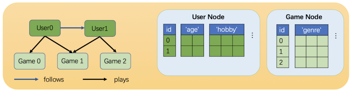
在DGL中每条关系使用三元组来表示(source node type, edge type, destination node type)

>>> import dgl
>>> import torch as th

>>> # Create a heterograph with 3 node types and 3 edges types.
>>> graph_data = {
...    ('drug', 'interacts', 'drug'): (th.tensor([0, 1]), th.tensor([1, 2])),
...    ('drug', 'interacts', 'gene'): (th.tensor([0, 1]), th.tensor([2, 3])),
...    ('drug', 'treats', 'disease'): (th.tensor([1]), th.tensor([2]))
... }
>>> g = dgl.heterograph(graph_data)
>>> g.ntypes
['disease', 'drug', 'gene']
>>> g.etypes
['interacts', 'interacts', 'treats']
>>> g.canonical_etypes
[('drug', 'interacts', 'drug'),
 ('drug', 'interacts', 'gene'),
 ('drug', 'treats', 'disease')]

同构图和二部图是特殊的异构图

>>> # A homogeneous graph  头尾节点类型相同
>>> dgl.heterograph({('node_type', 'edge_type', 'node_type'): (u, v)})
>>> # A bipartite graph  
>>> dgl.heterograph({('source_type', 'edge_type', 'destination_type'): (u, v)})

图的结构（metagraph）

>>> g
Graph(num_nodes={'disease': 3, 'drug': 3, 'gene': 4},
      num_edges={('drug', 'interacts', 'drug'): 2,
                 ('drug', 'interacts', 'gene'): 2,
                 ('drug', 'treats', 'disease'): 1},
      metagraph=[('drug', 'drug', 'interacts'),
                 ('drug', 'gene', 'interacts'),
                 ('drug', 'disease', 'treats')])
>>> g.metagraph().edges()
OutMultiEdgeDataView([('drug', 'drug'), ('drug', 'gene'), ('drug', 'disease')])

在dgl中不同类型的节点id是分开计数的，所以在使用nodes api时必须指定节点类型：

>>> # Get the number of all nodes in the graph
>>> g.num_nodes()
10
>>> # Get the number of drug nodes
>>> g.num_nodes('drug')
3
>>> # Nodes of different types have separate IDs,
>>> # hence not well-defined without a type specified
>>> g.nodes()
DGLError: Node type name must be specified if there are more than one node types.
>>> g.nodes('drug')
tensor([0, 1, 2])

设置和读取异构图中的节点特征和边特征：

>>> # Set/get feature 'hv' for nodes of type 'drug'
>>> g.nodes['drug'].data['hv'] = th.ones(3, 1)
>>> g.nodes['drug'].data['hv']
tensor([[1.],
        [1.],
        [1.]])
>>> # Set/get feature 'he' for edge of type 'treats'
>>> g.edges['treats'].data['he'] = th.zeros(1, 1)
>>> g.edges['treats'].data['he']
tensor([[0.]])

当只有一种节点类型时，就不用指定：

>>> g = dgl.heterograph({
...    ('drug', 'interacts', 'drug'): (th.tensor([0, 1]), th.tensor([1, 2])),
...    ('drug', 'is similar', 'drug'): (th.tensor([0, 1]), th.tensor([2, 3]))
... })
>>> g.nodes()
tensor([0, 1, 2, 3])
>>> # To set/get feature with a single type, no need to use the new syntax
>>> g.ndata['hv'] = th.ones(4, 1)

通过指定特定的关系，从异构图中创建子图：

>>> g = dgl.heterograph({
...    ('drug', 'interacts', 'drug'): (th.tensor([0, 1]), th.tensor([1, 2])),
...    ('drug', 'interacts', 'gene'): (th.tensor([0, 1]), th.tensor([2, 3])),
...    ('drug', 'treats', 'disease'): (th.tensor([1]), th.tensor([2]))
... })
>>> g.nodes['drug'].data['hv'] = th.ones(3, 1)

>>> # Retain relations ('drug', 'interacts', 'drug') and ('drug', 'treats', 'disease')
>>> # All nodes for 'drug' and 'disease' will be retained
>>> eg = dgl.edge_type_subgraph(g, [('drug', 'interacts', 'drug'),
...                                 ('drug', 'treats', 'disease')])
>>> eg
Graph(num_nodes={'disease': 3, 'drug': 3},
      num_edges={('drug', 'interacts', 'drug'): 2, ('drug', 'treats', 'disease'): 1},
      metagraph=[('drug', 'drug', 'interacts'), ('drug', 'disease', 'treats')])
>>> # The associated features will be copied as well
>>> eg.nodes['drug'].data['hv']
tensor([[1.],
        [1.],
        [1.]])

异构图转同构图：

>>> g = dgl.heterograph({
...    ('drug', 'interacts', 'drug'): (th.tensor([0, 1]), th.tensor([1, 2])),
...    ('drug', 'treats', 'disease'): (th.tensor([1]), th.tensor([2]))})
>>> g.nodes['drug'].data['hv'] = th.zeros(3, 1)
>>> g.nodes['disease'].data['hv'] = th.ones(3, 1)
>>> g.edges['interacts'].data['he'] = th.zeros(2, 1)
>>> g.edges['treats'].data['he'] = th.zeros(1, 2)

>>> # By default, it does not merge any features
>>> hg = dgl.to_homogeneous(g)
>>> 'hv' in hg.ndata
False

>>> # Copy edge features
>>> # For feature copy, it expects features to have
>>> # the same size and dtype across node/edge types
>>> hg = dgl.to_homogeneous(g, edata=['he'])
DGLError: Cannot concatenate column ‘he’ with shape Scheme(shape=(2,), dtype=torch.float32) and shape Scheme(shape=(1,), dtype=torch.float32)

>>> # Copy node features
>>> hg = dgl.to_homogeneous(g, ndata=['hv'])
>>> hg.ndata['hv']
tensor([[1.],
        [1.],
        [1.],
        [0.],
        [0.],
        [0.]])

The original node/edge types and type-specific IDs are stored in :py:attr:`~dgl.DGLGraph.ndata` and :py:attr:`~dgl.DGLGraph.edata`.

查看转换后同构图里节点和边在原异构图中的ID和类型：

>>> # Order of node types in the heterograph
>>> g.ntypes
['disease', 'drug']
>>> # Original node types
>>> hg.ndata[dgl.NTYPE]
tensor([0, 0, 0, 1, 1, 1])
>>> # Original type-specific node IDs
>>> hg.ndata[dgl.NID]
>>> tensor([0, 1, 2, 0, 1, 2])

>>> # Order of edge types in the heterograph
>>> g.etypes
['interacts', 'treats']
>>> # Original edge types
>>> hg.edata[dgl.ETYPE]
tensor([0, 0, 1])
>>> # Original type-specific edge IDs
>>> hg.edata[dgl.EID]
tensor([0, 1, 0])

1.6 在GPU上使用DGL

>>> import dgl
>>> import torch as th
>>> u, v = th.tensor([0, 1, 2]), th.tensor([2, 3, 4])
>>> g = dgl.graph((u, v))
>>> g.ndata['x'] = th.randn(5, 3)  # original feature is on CPU
>>> g.device
device(type='cpu')
>>> cuda_g = g.to('cuda:0')  # accepts any device objects from backend framework
>>> cuda_g.device
device(type='cuda', index=0)
>>> cuda_g.ndata['x'].device       # feature data is copied to GPU too
device(type='cuda', index=0)

>>> # A graph constructed from GPU tensors is also on GPU
>>> u, v = u.to('cuda:0'), v.to('cuda:0')
>>> g = dgl.graph((u, v))
>>> g.device
device(type='cuda', index=0)

CPU上的tensor不能传给GPU上的图，只能先把数据复制到同一设备：

>>> cuda_g.in_degrees()
tensor([0, 0, 1, 1, 1], device='cuda:0')
>>> cuda_g.in_edges([2, 3, 4])   # ok for non-tensor type arguments
(tensor([0, 1, 2], device='cuda:0'), tensor([2, 3, 4], device='cuda:0'))
>>> cuda_g.in_edges(th.tensor([2, 3, 4]).to('cuda:0'))  # tensor type must be on GPU
(tensor([0, 1, 2], device='cuda:0'), tensor([2, 3, 4], device='cuda:0'))
>>> cuda_g.ndata['h'] = th.randn(5, 4)  # ERROR! feature must be on GPU too!
DGLError: Cannot assign node feature "h" on device cpu to a graph on device
cuda:0. Call DGLGraph.to() to copy the graph to the same device.

Chapter 2: Message Passing

消息传递的范式

(x_vinmathbb{R}^{d_1})是节点(v)的特征，(w_{e}inmathbb{R}^{d_2})是边(({u}, {v}))的特征，边和节点的消息聚合范式如下：

[ ext{Edge-wise: } m_{e}^{(t+1)} = phi left( x_v^{(t)}, x_u^{(t)}, w_{e}^{(t)} ight) , ({u}, {v},{e}) in mathcal{E}.]

[ ext{Node-wise: } x_v^{(t+1)} = psi left(x_v^{(t)}, holeft(leftlbrace m_{e}^{(t+1)} : ({u}, {v},{e}) in mathcal{E} ight brace ight) ight). ]

其中(phi)是边上的消息函数，(psi)是更新函数函数，( ho)是聚合函数。(phi)决定着使用节点和边的特征生产何种消息，( ho)决定着对邻居节点传来的消息如何聚合，(psi)决定着如何利用第t步的值来对第t+1步进行更新。

DGL中内建的消息传播范式

在dgl.function空间下，DGL实现了常用的消息函数（message functions）和聚合函数（reduce functions），这些自带的函数已经进行了大量的优化，推荐优先使用。
目前内建消息函数支持一元运算支持：copy，二元运算支持：add，sub，mul，div，dot
除了内建函数，也可以自定义消息函数和聚合函数（UDF），命名规范通常是用u代表起点，v代表终点，e代表边。例如要实现将起点的hu特征加上终点的hv特征，最后传给边的he特征：

# 内建函数
dgl.function.u_add_v('hu', 'hv', 'he')
# UDF
def message_func(edges):
     return {'he': edges.src['hu'] + edges.dst['hv']}

目前内建的聚合函数支持：sum，max，min，prod，mean。reduce函数通常有两个参数：mailbox和dst。例如：

# 内建聚合函数
dgl.function.sum('m', 'h')
# UDF 
import torch
def reduce_func(nodes):
     return {'h': torch.sum(nodes.mailbox['m'], dim=1)}

# dgl中，对边的更新使用apply_edges()，需要传入一个消息函数
import dgl.function as fn
graph.apply_edges(fn.u_add_v('el', 'er', 'e'))

对节点的更新使用update_all()，需要消息函数、聚合函数和更新函数作为参数。

def updata_all_example(graph):
    # store the result in graph.ndata['ft']
    graph.update_all(fn.u_mul_e('ft', 'a', 'm'),
                    fn.sum('m', 'ft'))
    # Call update function outside of update_all
    final_ft = graph.ndata['ft'] * 2
    return final_ft

更新过程可以用数学公式表示为:({final\_ft}_i = 2 * sum_{jinmathcal{N}(i)} ({ft}_j * a_{ij}))

编写高效的消息传递代码

DGL对消息传递的内存消耗和运算速度都进行了优化：

• apply_edges 和update_all 矩阵乘法并行运算
• sampling out the node feature using entry index. (Memory and speed optimization)
• 对消息函数和聚合函数合并到一个运算单元，避免边上的消息处理过程。
  为了达到好的运算性能，推荐使用内建函数来组合自定义的消息传递过程。
  对于以下两种更新方式：

linear = nn.Parameter(th.FloatTensor(size=(1, node_feat_dim*2)))
def concat_message_function(edges):
    {'cat_feat': torch.cat([edges.src.ndata['feat'], edges.dst.ndata['feat']])}
g.apply_edges(concat_message_function)
g.edata['out'] = g.edata['cat_feat'] * linear

linear = nn.Parameter(th.FloatTensor(size=(1, node_feat_dim*2)))
def concat_message_function(edges):
    {'cat_feat': torch.cat([edges.src.ndata['feat'], edges.dst.ndata['feat']])}
g.apply_edges(concat_message_function)
g.edata['out'] = g.edata['cat_feat'] * linear

虽然结果都一样，但是第二种比一种运算时更高效，因为通常边的数量会远大于节点的数量，而第二种减少了将中间结果保存在边上的过程，从而减少了内存消耗。

在子图上进行消息传递

nid = [0, 2, 3, 6, 7, 9]
sg = g.subgraph(nid)
sg.update_all(message_func, reduce_func, apply_node_func)

在小批量迭代训练过程中，经常会使用子图的消息传递。

在消息传递过程中加入边的权值

graph.edata['a'] = affinity
graph.update_all(fn.u_mul_e('ft', 'a', 'm'),
                 fn.sum('m', 'ft'))

异构图上的消息传递

for c_etype in G.canonical_etypes:
    srctype, etype, dsttype = c_etype
    Wh = self.weight[etype](feat_dict[srctype])
    # Save it in graph for message passing
    G.nodes[srctype].data['Wh_%s' % etype] = Wh
    # Specify per-relation message passing functions: (message_func, reduce_func).
    # Note that the results are saved to the same destination feature 'h', which
    # hints the type wise reducer for aggregation.
    funcs[etype] = (fn.copy_u('Wh_%s' % etype, 'm'), fn.mean('m', 'h'))
# Trigger message passing of multiple types.
G.multi_update_all(funcs, 'sum')
# return the updated node feature dictionary
return {ntype : G.nodes[ntype].data['h'] for ntype in G.ntypes}

Chapter 3: Building GNN Modules

传统的深度学习网络模型中的输入和参数的维度都是固定的，但是在GNN网络中，每个节点的邻居个数可能是不一样的，因此需要做一些特殊的处理，需要将数据维度处理成固定的维度。DGL的作用在于对图数据结构的提供一些便利的操作方法。通常会使用DGL来处理处理图中节点和边的消息传递过程，而对应的tensor运算由pytorch和tensorflow等框架完成。

DGL nn模块的构造函数

指定输出，输出和隐藏层的维度，包括源节点和目的节点的维度。
设置不同边上的消息聚合方法：mean，sum，max， min，lstm。
正则化方法，例如l2正则：(h_v = h_v / lVert h_v Vert_2)

import torch as th
from torch import nn
from torch.nn import init

from .... import function as fn
from ....base import DGLError
from ....utils import expand_as_pair, check_eq_shape

class SAGEConv(nn.Module):
    def __init__(self,
                 in_feats,
                 out_feats,
                 aggregator_type,
                 bias=True,
                 norm=None,
                 activation=None):
        super(SAGEConv, self).__init__()

        self._in_src_feats, self._in_dst_feats = expand_as_pair(in_feats)
        self._out_feats = out_feats
        self._aggre_type = aggregator_type
        self.norm = norm
        self.activation = activation

不同的消息聚合方式实现，使用reset_parameters()方法进行参数初始化

def reset_parameters(self):
    """Reinitialize learnable parameters."""
    gain = nn.init.calculate_gain('relu')
    if self._aggre_type == 'max_pool':
        nn.init.xavier_uniform_(self.fc_pool.weight, gain=gain)
    if self._aggre_type == 'lstm':
        self.lstm.reset_parameters()
    if self._aggre_type != 'gcn':
        nn.init.xavier_uniform_(self.fc_self.weight, gain=gain)
    nn.init.xavier_uniform_(self.fc_neigh.weight, gain=gain)

# aggregator type: mean, max_pool, lstm, gcn
if aggregator_type not in ['mean', 'max_pool', 'lstm', 'gcn']:
    raise KeyError('Aggregator type {} not supported.'.format(aggregator_type))
if aggregator_type == 'max_pool':
    self.fc_pool = nn.Linear(self._in_src_feats, self._in_src_feats)
if aggregator_type == 'lstm':
    self.lstm = nn.LSTM(self._in_src_feats, self._in_src_feats, batch_first=True)
if aggregator_type in ['mean', 'max_pool', 'lstm']:
    self.fc_self = nn.Linear(self._in_dst_feats, out_feats, bias=bias)
self.fc_neigh = nn.Linear(self._in_src_feats, out_feats, bias=bias)
self.reset_parameters()

DGL nn模块的前向计算方法

def forward(self, graph, feat):
    with graph.local_scope():
        # Specify graph type then expand input feature according to graph type
        feat_src, feat_dst = expand_as_pair(feat, graph)

SAGEConv的过程可以用数学公式表示为：

[h_{mathcal{N}(dst)}^{(l+1)} = mathrm{aggregate} left({h_{src}^{l}, forall src in mathcal{N}(dst) } ight) ]

[h_{dst}^{(l+1)} = sigma left(W cdot mathrm{concat} (h_{dst}^{l}, h_{mathcal{N}(dst)}^{l+1} + b) ight) ]

[h_{dst}^{(l+1)} = mathrm{norm}(h_{dst}^{l}) ]

在同构图中，整个训练过程的源节点和目的节点的类型是相同的。
而在异构图的训练过程中，可以被分成多种二部图，每个二部图对应了一种节点之间的关系（src_type, edge_type, dst_dtype）。在批量训练中，每次的训练过程只发生在叫做block的子图上，只有在block中的目的节点会根据传递的消息进行更新。

SAGEConv 的消息传递和聚合

if self._aggre_type == 'mean':
    graph.srcdata['h'] = feat_src
    graph.update_all(fn.copy_u('h', 'm'), fn.mean('m', 'neigh'))
    h_neigh = graph.dstdata['neigh']
elif self._aggre_type == 'gcn':
    check_eq_shape(feat)
    graph.srcdata['h'] = feat_src
    graph.dstdata['h'] = feat_dst     # same as above if homogeneous
    graph.update_all(fn.copy_u('h', 'm'), fn.sum('m', 'neigh'))
    # divide in_degrees
    degs = graph.in_degrees().to(feat_dst)
    h_neigh = (graph.dstdata['neigh'] + graph.dstdata['h']) / (degs.unsqueeze(-1) + 1)
elif self._aggre_type == 'max_pool':
    graph.srcdata['h'] = F.relu(self.fc_pool(feat_src))
    graph.update_all(fn.copy_u('h', 'm'), fn.max('m', 'neigh'))
    h_neigh = graph.dstdata['neigh']
else:
    raise KeyError('Aggregator type {} not recognized.'.format(self._aggre_type))

# GraphSAGE GCN does not require fc_self.
if self._aggre_type == 'gcn':
    rst = self.fc_neigh(h_neigh)
else:
    rst = self.fc_self(h_self) + self.fc_neigh(h_neigh)

激活函数和正则

# activation
if self.activation is not None:
    rst = self.activation(rst)
# normalization
if self.norm is not None:
    rst = self.norm(rst)
return rst

y异构图中的GraphConv 模块

异构图中的GraphConv 可以表示为：

[h_{dst}^{(l+1)} = underset{rinmathcal{R}, r_{dst}=dst}{AGG} (f_r(g_r, h_{r_{src}}^l, h_{r_{dst}}^l)) ]

其中(f_r)表示处理关系(r)的模块。

class HeteroGraphConv(nn.Module):
    def __init__(self, mods, aggregate='sum'):
        super(HeteroGraphConv, self).__init__()
        self.mods = nn.ModuleDict(mods)
        if isinstance(aggregate, str):
            self.agg_fn = get_aggregate_fn(aggregate)
        else:
            self.agg_fn = aggregate
    def forward(self, g, inputs, mod_args=None, mod_kwargs=None):
        if mod_args is None:
            mod_args = {}
        if mod_kwargs is None:
            mod_kwargs = {}
        outputs = {nty : [] for nty in g.dsttypes}

    if g.is_block:
        src_inputs = inputs
        dst_inputs = {k: v[:g.number_of_dst_nodes(k)] for k, v in inputs.items()}
    else:
        src_inputs = dst_inputs = inputs

    for stype, etype, dtype in g.canonical_etypes:
        rel_graph = g[stype, etype, dtype]
        if rel_graph.number_of_edges() == 0:
            continue
        if stype not in src_inputs or dtype not in dst_inputs:
            continue
        dstdata = self.mods[etype](
                        rel_graph,
                        (src_inputs[stype], dst_inputs[dtype]),
                        *mod_args.get(etype, ()),
                        **mod_kwargs.get(etype, {}))
        outputs[dtype].append(dstdata)

rsts = {}
for nty, alist in outputs.items():
    if len(alist) != 0:
        rsts[nty] = self.agg_fn(alist, nty)

Chapter 4: Graph Data Pipeline

DGL 中主要使用dgl.data.DGLDataset子类来数据进行读取、处理和保存图数据。
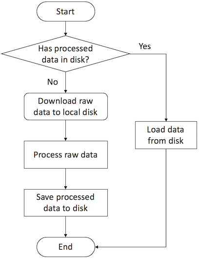
DGLDataset类定义的数据处理流程：

例如：下面是一个数据读取的模板

from dgl.data import DGLDataset

class MyDataset(DGLDataset):
    """ Template for customizing graph datasets in DGL.

    Parameters
    ----------
    url : str
        URL to download the raw dataset
    raw_dir : str
        Specifying the directory that will store the
        downloaded data or the directory that
        already stores the input data.
        Default: ~/.dgl/
    save_dir : str
        Directory to save the processed dataset.
        Default: the value of `raw_dir`
    force_reload : bool
        Whether to reload the dataset. Default: False
    verbose : bool
        Whether to print out progress information
    """
    def __init__(self,
                 url=None,
                 raw_dir=None,
                 save_dir=None,
                 force_reload=False,
                 verbose=False):
        super(MyDataset, self).__init__(name='dataset_name',
                                        url=url,
                                        raw_dir=raw_dir,
                                        save_dir=save_dir,
                                        force_reload=force_reload,
                                        verbose=verbose)

    def download(self):
        # download raw data to local disk
        pass

    def process(self):
        # process raw data to graphs, labels, splitting masks
        pass

    def __getitem__(self, idx):
        # get one example by index
        pass

    def __len__(self):
        # number of data examples
        pass

    def save(self):
        # save processed data to directory `self.save_path`
        pass

    def load(self):
        # load processed data from directory `self.save_path`
        pass

    def has_cache(self):
        # check whether there are processed data in `self.save_path`
        pass

Download raw data (optional)

from dgl.data.utils import download, extract_archive

def download(self):
    # path to store the file
    # make sure to use the same suffix as the original file name's
    gz_file_path = os.path.join(self.raw_dir, self.name + '.csv.gz')
    # download file
    download(self.url, path=gz_file_path)
    # check SHA-1
    if not check_sha1(gz_file_path, self._sha1_str):
        raise UserWarning('File {} is downloaded but the content hash does not match.'
                          'The repo may be outdated or download may be incomplete. '
                          'Otherwise you can create an issue for it.'.format(self.name + '.csv.gz'))
    # extract file to directory `self.name` under `self.raw_dir`
    self._extract_gz(gz_file_path, self.raw_path)

Process data

Processing Graph Classification datasets

Processing Node Classification datasets

Processing dataset for Link Prediction datasets

Save and load data

Loading OGB datasets using ogb package

Chapter 5: Training Graph Neural Networks

在图神经网络中，一般有节点分类、边分类、边预测（两个节点存在边的可能性）、对图作为一个整体的分类等任务。
首先用人工生成的异构图作为例子，图中的边类型有：
('user', 'follow', 'user')
('user', 'followed-by', 'user')
('user', 'click', 'item')
('item', 'clicked-by', 'user')
('user', 'dislike', 'item')
('item', 'disliked-by', 'user')
构造异构图的代码如下：

import numpy as np
import torch

n_users = 1000
n_items = 500
n_follows = 3000
n_clicks = 5000
n_dislikes = 500
n_hetero_features = 10
n_user_classes = 5
n_max_clicks = 10

follow_src = np.random.randint(0, n_users, n_follows)
follow_dst = np.random.randint(0, n_users, n_follows)
click_src = np.random.randint(0, n_users, n_clicks)
click_dst = np.random.randint(0, n_items, n_clicks)
dislike_src = np.random.randint(0, n_users, n_dislikes)
dislike_dst = np.random.randint(0, n_items, n_dislikes)

hetero_graph = dgl.heterograph({
    ('user', 'follow', 'user'): (follow_src, follow_dst),
    ('user', 'followed-by', 'user'): (follow_dst, follow_src),
    ('user', 'click', 'item'): (click_src, click_dst),
    ('item', 'clicked-by', 'user'): (click_dst, click_src),
    ('user', 'dislike', 'item'): (dislike_src, dislike_dst),
    ('item', 'disliked-by', 'user'): (dislike_dst, dislike_src)})

hetero_graph.nodes['user'].data['feature'] = torch.randn(n_users, n_hetero_features)
hetero_graph.nodes['item'].data['feature'] = torch.randn(n_items, n_hetero_features)
hetero_graph.nodes['user'].data['label'] = torch.randint(0, n_user_classes, (n_users,))
hetero_graph.edges['click'].data['label'] = torch.randint(1, n_max_clicks, (n_clicks,)).float()
# randomly generate training masks on user nodes and click edges
hetero_graph.nodes['user'].data['train_mask'] = torch.zeros(n_users, dtype=torch.bool).bernoulli(0.6)
hetero_graph.edges['click'].data['train_mask'] = torch.zeros(n_clicks, dtype=torch.bool).bernoulli(0.6)

5.1 Node Classification/Regression

模型定义：

# Contruct a two-layer GNN model
import dgl.nn as dglnn
import torch.nn as nn
import torch.nn.functional as F
class SAGE(nn.Module):
    def __init__(self, in_feats, hid_feats, out_feats):
        super().__init__()
        self.conv1 = dglnn.SAGEConv(
            in_feats=in_feats, out_feats=hid_feats, aggregator_type='mean')
        self.conv2 = dglnn.SAGEConv(
            in_feats=hid_feats, out_feats=out_feats, aggregator_type='mean')

    def forward(self, graph, inputs):
        # inputs are features of nodes
        h = self.conv1(graph, inputs)
        h = F.relu(h)
        h = self.conv2(graph, h)
        return h
def evaluate(model, graph, features, labels, mask):
    model.eval()
    with torch.no_grad():
        logits = model(graph, features)
        logits = logits[mask]
        labels = labels[mask]
        _, indices = torch.max(logits, dim=1)
        correct = torch.sum(indices == labels)
        return correct.item() * 1.0 / len(labels)

训练流程：

node_features = graph.ndata['feat']
node_labels = graph.ndata['label']
train_mask = graph.ndata['train_mask']
valid_mask = graph.ndata['val_mask']
test_mask = graph.ndata['test_mask']
n_features = node_features.shape[1]
n_labels = int(node_labels.max().item() + 1)
model = SAGE(in_feats=n_features, hid_feats=100, out_feats=n_labels)
opt = torch.optim.Adam(model.parameters())

for epoch in range(10):
    model.train()
    # forward propagation by using all nodes
    logits = model(graph, node_features)
    # compute loss
    loss = F.cross_entropy(logits[train_mask], node_labels[train_mask])
    # compute validation accuracy
    acc = evaluate(model, graph, node_features, node_labels, valid_mask)
    # backward propagation
    opt.zero_grad()
    loss.backward()
    opt.step()
    print(loss.item())

    # Save model if necessary.  Omitted in this example.

异构图的训练过程：

# Define a Heterograph Conv model
import dgl.nn as dglnn

class RGCN(nn.Module):
    def __init__(self, in_feats, hid_feats, out_feats, rel_names):
        super().__init__()

        self.conv1 = dglnn.HeteroGraphConv({
            rel: dglnn.GraphConv(in_feats, hid_feats)
            for rel in rel_names}, aggregate='sum')
        self.conv2 = dglnn.HeteroGraphConv({
            rel: dglnn.GraphConv(hid_feats, out_feats)
            for rel in rel_names}, aggregate='sum')

    def forward(self, graph, inputs):
        # inputs are features of nodes
        h = self.conv1(graph, inputs)
        h = {k: F.relu(v) for k, v in h.items()}
        h = self.conv2(graph, h)
        return h

model = RGCN(n_hetero_features, 20, n_user_classes, hetero_graph.etypes)
user_feats = hetero_graph.nodes['user'].data['feature']
item_feats = hetero_graph.nodes['item'].data['feature']
labels = hetero_graph.nodes['user'].data['label']
train_mask = hetero_graph.nodes['user'].data['train_mask']
opt = torch.optim.Adam(model.parameters())

for epoch in range(5):
    model.train()
    # forward propagation by using all nodes and extracting the user embeddings
    logits = model(hetero_graph, node_features)['user']
    # compute loss
    loss = F.cross_entropy(logits[train_mask], labels[train_mask])
    # Compute validation accuracy.  Omitted in this example.
    # backward propagation
    opt.zero_grad()
    loss.backward()
    opt.step()
    print(loss.item())

    # Save model if necessary.  Omitted in the example.

当只需要进行推理时：

node_features = {'user': user_feats, 'item': item_feats}
h_dict = model(hetero_graph, {'user': user_feats, 'item': item_feats})
h_user = h_dict['user']
h_item = h_dict['item']

5.2 Edge Classification/Regression

在一些任务中，可能需要对边上的属性进行预测或者可能需要预测两个节点之间是否存在边，这时就涉及到了边的分类（回归任务）。
首先随机生成一下数据：

src = np.random.randint(0, 100, 500)
dst = np.random.randint(0, 100, 500)
# make it symmetric
edge_pred_graph = dgl.graph((np.concatenate([src, dst]), np.concatenate([dst, src])))
# synthetic node and edge features, as well as edge labels
edge_pred_graph.ndata['feature'] = torch.randn(100, 10)
edge_pred_graph.edata['feature'] = torch.randn(1000, 10)
edge_pred_graph.edata['label'] = torch.randn(1000)
# synthetic train-validation-test splits
edge_pred_graph.edata['train_mask'] = torch.zeros(1000, dtype=torch.bool).bernoulli(0.6)

边的分类和回归任务与节点分类任务类似，也是需要计算节点的嵌入表示，然后利用节点的表示，计算边的类别或者边上的score。
例如：可以使用如下方式直接使用节点的表示向量h来计算边的回归值。

import dgl.function as fn
class DotProductPredictor(nn.Module):
    def forward(self, graph, h):
        # h contains the node representations computed from the GNN defined
        # in the node classification section (Section 5.1).
        with graph.local_scope():
            graph.ndata['h'] = h
            graph.apply_edges(fn.u_dot_v('h', 'h', 'score'))
            return graph.edata['score']

另外，也可以使用自己定义一个apply_edges()方法，来实现不同的计算过程：

class MLPPredictor(nn.Module):
    def __init__(self, in_features, out_classes):
        super().__init__()
        self.W = nn.Linear(in_features * 2, out_classes)

    def apply_edges(self, edges):
        h_u = edges.src['h']
        h_v = edges.dst['h']
        score = self.W(torch.cat([h_u, h_v], 1))
        return {'score': score}

    def forward(self, graph, h):
        # h contains the node representations computed from the GNN defined
        # in the node classification section (Section 5.1).
        with graph.local_scope():
            graph.ndata['h'] = h
            graph.apply_edges(self.apply_edges)
            return graph.edata['score']

全图训练的流程：

class Model(nn.Module):
    def __init__(self, in_features, hidden_features, out_features):
        super().__init__()
        self.sage = SAGE(in_features, hidden_features, out_features)
        self.pred = DotProductPredictor()
    def forward(self, g, x):
        h = self.sage(g, x)
        return self.pred(g, h)

node_features = edge_pred_graph.ndata['feature']
edge_label = edge_pred_graph.edata['label']
train_mask = edge_pred_graph.edata['train_mask']
model = Model(10, 20, 5)
opt = torch.optim.Adam(model.parameters())
for epoch in range(10):
    pred = model(edge_pred_graph, node_features)
    loss = ((pred[train_mask] - edge_label[train_mask]) ** 2).mean()
    opt.zero_grad()
    loss.backward()
    opt.step()
    print(loss.item())

对于异构图，也是类似的，只需要在apply_edges函数中加入etype参数，指定边的类型：

#### 直接使用节点表示，计算点积
class HeteroDotProductPredictor(nn.Module):
    def forward(self, graph, h, etype):
        # h contains the node representations for each edge type computed from
        # the GNN for heterogeneous graphs defined in the node classification
        # section (Section 5.1).
        with graph.local_scope():
            graph.ndata['h'] = h   # assigns 'h' of all node types in one shot
            graph.apply_edges(fn.u_dot_v('h', 'h', 'score'), etype=etype)
            return graph.edges[etype].data['score']

#### 自定义 edges score计算方式
class MLPPredictor(nn.Module):
    def __init__(self, in_features, out_classes):
        super().__init__()
        self.W = nn.Linear(in_features * 2, out_classes)

    def apply_edges(self, edges):
        h_u = edges.src['h']
        h_v = edges.dst['h']
        score = self.W(torch.cat([h_u, h_v], 1))
        return {'score': score}

    def forward(self, graph, h, etype):
        # h contains the node representations for each edge type computed from
        # the GNN for heterogeneous graphs defined in the node classification
        # section (Section 5.1).
        with graph.local_scope():
            graph.ndata['h'] = h   # assigns 'h' of all node types in one shot
            graph.apply_edges(self.apply_edges, etype=etype)
            return graph.edges[etype].data['score']

异构图的全图训练流程如下：

class Model(nn.Module):
    def __init__(self, in_features, hidden_features, out_features, rel_names):
        super().__init__()
        self.sage = RGCN(in_features, hidden_features, out_features, rel_names)
        self.pred = HeteroDotProductPredictor()
    def forward(self, g, x, etype):
        h = self.sage(g, x)
        return self.pred(g, h, etype)

model = Model(10, 20, 5, hetero_graph.etypes)
user_feats = hetero_graph.nodes['user'].data['feature']
item_feats = hetero_graph.nodes['item'].data['feature']
label = hetero_graph.edges['click'].data['label']
train_mask = hetero_graph.edges['click'].data['train_mask']
node_features = {'user': user_feats, 'item': item_feats}

opt = torch.optim.Adam(model.parameters())
for epoch in range(10):
    pred = model(hetero_graph, node_features, 'click')
    loss = ((pred[train_mask] - label[train_mask]) ** 2).mean()
    opt.zero_grad()
    loss.backward()
    opt.step()
    print(loss.item())

5.3 Link Prediction

有时需要对给定的两个节点预测，节点间是否存在一条边。仍然是利用两个节点的表示建模：

[y_{u,v} = phi(oldsymbol{h}_u^{(L)}, oldsymbol{h}_v^{(L)}) ]

在训练过程中，一般采用加入负采样的损失函数。
Cross-entropy loss:(mathcal{L} = - log sigma (y_{u,v}) - sum_{v_i sim P_n(v), i=1,dots,k}log left[ 1 - sigma (y_{u,v_i}) ight])
BPR loss: (mathcal{L} = sum_{v_i sim P_n(v), i=1,dots,k} - log sigma (y_{u,v} - y_{u,v_i}))
Margin loss: (mathcal{L} = sum_{v_i sim P_n(v), i=1,dots,k} max(0, M - y_{u, v} + y_{u, v_i}))，其中M是一个超参数。

class DotProductPredictor(nn.Module):
    def forward(self, graph, h):
        # h contains the node representations computed from the GNN defined
        # in the node classification section (Section 5.1).
        with graph.local_scope():
            graph.ndata['h'] = h
            graph.apply_edges(fn.u_dot_v('h', 'h', 'score'))
            return graph.edata['score']

def construct_negative_graph(graph, k):
    src, dst = graph.edges()

    neg_src = src.repeat_interleave(k)
    neg_dst = torch.randint(0, graph.number_of_nodes(), (len(src) * k,))
    return dgl.graph((neg_src, neg_dst), num_nodes=graph.number_of_nodes())

class Model(nn.Module):
    def __init__(self, in_features, hidden_features, out_features):
        super().__init__()
        self.sage = SAGE(in_features, hidden_features, out_features)
        self.pred = DotProductPredictor()
    def forward(self, g, neg_g, x):
        h = self.sage(g, x)
        return self.pred(g, h), self.pred(neg_g, h)
def compute_loss(pos_score, neg_score):
    # Margin loss
    n_edges = pos_score.shape[0]
    return (1 - neg_score.view(n_edges, -1) + pos_score.unsqueeze(1)).clamp(min=0).mean()

node_features = graph.ndata['feat']
n_features = node_features.shape[1]
k = 5
model = Model(n_features, 100, 100)
opt = torch.optim.Adam(model.parameters())
for epoch in range(10):
    negative_graph = construct_negative_graph(graph, k)
    pos_score, neg_score = model(graph, negative_graph, node_features)
    loss = compute_loss(pos_score, neg_score)
    opt.zero_grad()
    loss.backward()
    opt.step()
    print(loss.item())

训练完成后
node_embeddings = model.sage(graph, node_features)
然后使用两个节点的嵌入表示计算节点之间存在边的概率。
在异构图的训练过程如下：

class HeteroDotProductPredictor(nn.Module):
    def forward(self, graph, h, etype):
        # h contains the node representations for each node type computed from
        # the GNN defined in the previous section (Section 5.1).
        with graph.local_scope():
            graph.ndata['h'] = h
            graph.apply_edges(fn.u_dot_v('h', 'h', 'score'), etype=etype)
            return graph.edges[etype].data['score']

def construct_negative_graph(graph, k, etype):
    utype, _, vtype = etype
    src, dst = graph.edges(etype=etype)
    neg_src = src.repeat_interleave(k)
    neg_dst = torch.randint(0, graph.number_of_nodes(vtype), (len(src) * k,))
    return dgl.heterograph(
        {etype: (neg_src, neg_dst)},
        num_nodes_dict={ntype: graph.number_of_nodes(ntype) for ntype in graph.ntypes})

class Model(nn.Module):
    def __init__(self, in_features, hidden_features, out_features, rel_names):
        super().__init__()
        self.sage = RGCN(in_features, hidden_features, out_features, rel_names)
        self.pred = HeteroDotProductPredictor()
    def forward(self, g, neg_g, x, etype):
        h = self.sage(g, x)
        return self.pred(g, h, etype), self.pred(neg_g, h, etype)
def compute_loss(pos_score, neg_score):
    # Margin loss
    n_edges = pos_score.shape[0]
    return (1 - neg_score.view(n_edges, -1) + pos_score.unsqueeze(1)).clamp(min=0).mean()

k = 5
model = Model(10, 20, 5, hetero_graph.etypes)
user_feats = hetero_graph.nodes['user'].data['feature']
item_feats = hetero_graph.nodes['item'].data['feature']
node_features = {'user': user_feats, 'item': item_feats}
opt = torch.optim.Adam(model.parameters())
for epoch in range(10):
    negative_graph = construct_negative_graph(hetero_graph, k, ('user', 'click', 'item'))
    pos_score, neg_score = model(hetero_graph, negative_graph, node_features, ('user', 'click', 'item'))
    loss = compute_loss(pos_score, neg_score)
    opt.zero_grad()
    loss.backward()
    opt.step()
    print(loss.item())

Chapter 6: Stochastic Training on Large Graphs

在实际使用中，如果边或节点数超过百万甚至是十亿级别的时候，就无法使用上一章介绍的在全图上的训练流程了。假设network layer为L，隐藏层的维度为H，节点的个数为N，此时需要的空间为：O(NLH)，如果N的值很大，很容易就会超过GPU的内存。因此需要使用批梯度下降训练，主要采用的邻居抽样的方法：

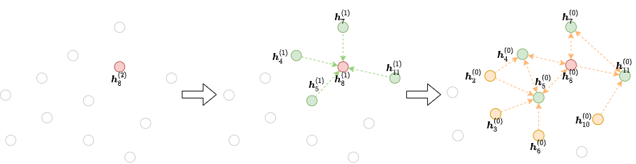
节点分类中的邻居采样

import dgl
import dgl.nn as dglnn
import torch
import torch.nn as nn
import torch.nn.functional as F

sampler = dgl.dataloading.MultiLayerFullNeighborSampler(2)
dataloader = dgl.dataloading.NodeDataLoader(
    g, train_nids, sampler,
    batch_size=1024,
    shuffle=True,
    drop_last=False,
    num_workers=4)

dataloader 每个批次返回3个对象；input_nodes, output_nodes, blocks。input_nodes对应了这个批次所有涉及的节点，output_nodes是批次里最后需要表示的节点，blocks里描述了批次里节点之间的连接关系。
模型定义如下：

## 全图训练的模型定义：
class TwoLayerGCN(nn.Module):
    def __init__(self, in_features, hidden_features, out_features):
        super().__init__()
        self.conv1 = dglnn.GraphConv(in_features, hidden_features)
        self.conv2 = dglnn.GraphConv(hidden_features, out_features)

    def forward(self, g, x):
        x = F.relu(self.conv1(g, x))
        x = F.relu(self.conv2(g, x))
        return x

## 批次训练的模型定义：
class StochasticTwoLayerGCN(nn.Module):
    def __init__(self, in_features, hidden_features, out_features):
        super().__init__()
        self.conv1 = dgl.nn.GraphConv(in_features, hidden_features)
        self.conv2 = dgl.nn.GraphConv(hidden_features, out_features)

    def forward(self, blocks, x):
        x = F.relu(self.conv1(blocks[0], x))
        x = F.relu(self.conv2(blocks[1], x))
        return x

可以看到模型结构和参数是相同的，只是不同网络层传递的参数是不同的。
整个训练流程大致可以分为四个部分：
1、取出input nodes的特征复制到GPU
2、将input nodes特征和blocks输入到模型，接收模型的输出
3、取出label复制到GPU （1和3可以合并）
4、计算loss并反选传播损失

model = StochasticTwoLayerGCN(in_features, hidden_features, out_features)
model = model.cuda()
opt = torch.optim.Adam(model.parameters())

for input_nodes, output_nodes, blocks in dataloader:
    blocks = [b.to(torch.device('cuda')) for b in blocks]
    input_features = blocks[0].srcdata['features']
    output_labels = blocks[-1].dstdata['label']
    output_predictions = model(blocks, input_features)
    loss = compute_loss(output_labels, output_predictions)
    opt.zero_grad()
    loss.backward()
    opt.step()

异构图的训练：

class StochasticTwoLayerRGCN(nn.Module):
    def __init__(self, in_feat, hidden_feat, out_feat):
        super().__init__()
        self.conv1 = dglnn.HeteroGraphConv({
                rel : dglnn.GraphConv(in_feat, hidden_feat, norm='right')
                for rel in rel_names
            })
        self.conv2 = dglnn.HeteroGraphConv({
                rel : dglnn.GraphConv(hidden_feat, out_feat, norm='right')
                for rel in rel_names
            })

    def forward(self, blocks, x):
        x = self.conv1(blocks[0], x)
        x = self.conv2(blocks[1], x)
        return x

sampler = dgl.dataloading.MultiLayerFullNeighborSampler(2)
dataloader = dgl.dataloading.NodeDataLoader(
    g, train_nid_dict, sampler,
    batch_size=1024,
    shuffle=True,
    drop_last=False,
    num_workers=4)

model = StochasticTwoLayerRGCN(in_features, hidden_features, out_features)
model = model.cuda()
opt = torch.optim.Adam(model.parameters())

for input_nodes, output_nodes, blocks in dataloader:
    blocks = [b.to(torch.device('cuda')) for b in blocks]
    input_features = blocks[0].srcdata     # returns a dict
    output_labels = blocks[-1].dstdata     # returns a dict
    output_predictions = model(blocks, input_features)
    loss = compute_loss(output_labels, output_predictions)
    opt.zero_grad()
    loss.backward()
    opt.step()