局部加权线性回归
【转载时请注明来源】:http://www.cnblogs.com/runner-ljt/
Ljt
作为一个初学者,水平有限,欢迎交流指正。
线性回归容易出现过拟合或欠拟合的问题。
局部加权线性回归是一种非参数学习方法,在对新样本进行预测时,会根据新的权值,重新训练样本数据得到新的参数值,每一次预测的参数值是不相同的。
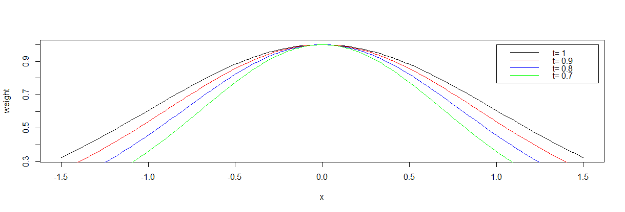
权值函数:

t用来控制权值的变化速率(建议对于不同的样本,先通过调整t值确定合适的t)
不同t值下的权值函数图像:
局部加权线性回归R实现:
#Locally Weighted Linear Regression 局部加权回归(非参数学习方法)

##x为数据矩阵(mxn m:样本数 n:特征数 );y观测值(mx1);xp为需要预测的样本特征,t权重函数的权值变化速率
#error终止条件,相邻两次搜索结果的幅度;
#step为设定的固定步长;maxiter最大迭代次数,alpha,beta为回溯下降法的参数

LWLRegression<-function(x,y,xp,t,error,maxiter,stepmethod=T,step=0.001,alpha=0.25,beta=0.8)
{
  w<-exp(-0.5*(x-xp)^2./t^2)  #权重函数,w(i)表示第i个样本点的权重,t控制权重的变化速率
  m<-nrow(x)
  x<-cbind(matrix(1,m,1),x)
  n<-ncol(x)
  theta<-matrix(0,n,1)  #theta初始值都设置为0
  iter<-0
  newerror<-1

  while((newerror>error)|(iter<maxiter)){
  iter<-iter+1
  h<-x%*%theta
  des<-t(t(w*(h-y))%*%x)  #梯度

  #回溯下降法求步长t
  if(stepmethod==T){
    step=1
    new_theta<-theta-step*des
    new_h<-x%*%new_theta
    costfunction<-t(w*(h-y))%*%(h-y)  #(最小二乘损失函数)局部加权线性回归损失函数
    new_costfunction<-t(w*(new_h-y))%*%(new_h-y)
    #回溯下降法求步长step
    while(new_costfunction>costfunction-alpha*step*sum(des*des)){
      step<-step*beta
      new_theta<-theta-step*des
      new_h<-x%*%new_theta
      new_costfunction<-t(w*(new_h-y))%*%(new_h-y)
    }
    newerror<-t(theta-new_theta)%*%(theta-new_theta)
    theta<-new_theta
  }

  #直接设置固定步长
  if(stepmethod==F){
    new_theta<-theta-step*des
    newerror<-t(theta-new_theta)%*%(theta-new_theta)
    theta<-new_theta
  }
 }

  xp<-cbind(1,xp)
  yp<-xp%*%theta
  #costfunction<-t(x%*%theta-y)%*%(x%*%theta-y)
  #result<-list(yp,theta,iter,costfunction)
  #names(result)<-c('拟合值','系数','迭代次数','误差')
  #result
  yp
}
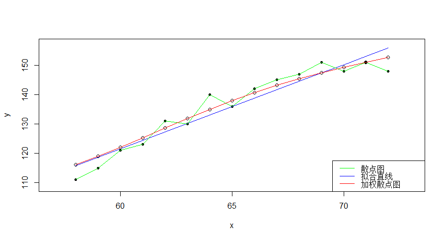
运用局部线性加权回归预测每个样本点x对于的y值,连接各预测值后得到一条平滑曲线,反映出y与x之间的非线性关系。
> t(x)
     [,1] [,2] [,3] [,4] [,5] [,6] [,7] [,8] [,9] [,10] [,11] [,12] [,13] [,14] [,15]
[1,]   58   59   60   61   62   63   64   65   66    67    68    69    70    71    72
> t(y)
     [,1] [,2] [,3] [,4] [,5] [,6] [,7] [,8] [,9] [,10] [,11] [,12] [,13] [,14] [,15]
[1,]  111  115  121  123  131  130  140  136  142   145   147   151   148   151   148
>
> lm(y~x)

Call:
lm(formula = y ~ x)

Coefficients:
(Intercept)            x
    -50.245        2.864

> yy<--50.245+2.864*x
> t(yy)
        [,1]    [,2]    [,3]    [,4]    [,5]    [,6]    [,7]    [,8]    [,9]   [,10]   [,11]   [,12]   [,13]   [,14]   [,15]
[1,] 115.867 118.731 121.595 124.459 127.323 130.187 133.051 135.915 138.779 141.643 144.507 147.371 150.235 153.099 155.963
>
> g<-apply(x,1,function(xp){LWLRegression(x,y,xp,3,1e-7,100000,stepmethod=F,step=0.00001,alpha=0.25,beta=0.8)})
>
> t(g)
        [,1]     [,2]     [,3]     [,4]     [,5]    [,6]    [,7]     [,8]     [,9]   [,10]    [,11]    [,12]    [,13]   [,14]
[1,] 116.093 119.0384 122.1318 125.3421 128.6115 131.862 135.009 137.9771 140.7136 143.194 145.4244 147.4373 149.2831 151.018
       [,15]
[1,] 152.693
>
> plot(x,y,pch=20,xlim=c(57,73),ylim=c(109,157))
> lines(x,y,col='green')
> lines(x,yy,col='blue')
> points(x,g,pch=21)
> lines(x,g,col='red')
> legend("bottomright",legend=c('散点图','拟合直线','加权散点图'),lwd=1,col=c('green','blue','red'))
>