下载数据
import os
import tarfile  # 用于压缩和解压文件
import urllib

DOWNLOAD_ROOT = "https://raw.githubusercontent.com/ageron/handson-ml/master/"
HOUSING_PATH = "datasets/housing"
HOUSING_URL = DOWNLOAD_ROOT + HOUSING_PATH + "/housing.tgz"


# 下载数据
def fetch_housing_data(housing_url=HOUSING_URL, housing_path=HOUSING_PATH):
    if not os.path.isdir(housing_path):
        os.makedirs(housing_path)
    tgz_path = os.path.join(housing_path, "housing.tgz")
    # urlretrieve()方法直接将远程数据下载到本地
    urllib.request.urlretrieve(housing_url, tgz_path)
    housing_tgz = tarfile.open(tgz_path)
    housing_tgz.extractall(path=housing_path)  # 解压文件到指定路径,不指定就是解压到当前路径
    housing_tgz.close()
fetch_housing_data()
加载数据
import pandas as pd

def load_housing_data(housing_path=HOUSING_PATH + "/"):
    csv_path = os.path.join(housing_path, "housing.csv")
    return pd.read_csv(csv_path)
housing = load_housing_data()
housing.head()
查看数据结构
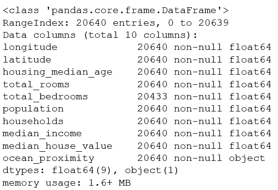
info()
info()方法可以快速查看数据的描述,特别是总行数、每个属性的类型和非空值的数量
housing.describe()
housing.info()
# 分析:数据集中共有 20640 个实例,按照机器学习的标准这个数据量很小,但是非常适合入门。
# 我们注意到总卧室数只有 20433 个非空值,这意味着有 207 个街区缺少这个值。我们将在后面对它进行处理。
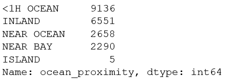
value_counts()
所有的属性都是数值的,除了离大海距离这项。它的类型是对象,因此可以包含任意 Python 对象,但是因为该项是从 CSV 文件加载的,所以必然是文本类型。在刚才查看数据前五项时,你可能注意到那一列的值是重复的,意味着它可能是一项表示类别的属性。可以使用value_counts()方法查看该项中都有哪些类别,每个类别中都包含有多少个街区:
housing["ocean_proximity"].value_counts()
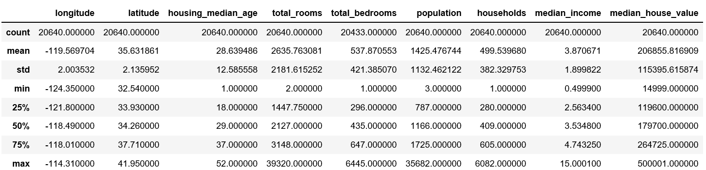
describe()
describe()方法展示了数值属性的概括
housing.describe()
图形描述
使用matplotlib的hist()将属性值画成柱状图,更直观
import matplotlib.pyplot as plt
housing.hist(bins=50, figsize=(10,10))
plt.show() # 不是必要的

- 房屋年龄中位数和房屋价值中位数也被设了上限,因此图中末尾为一条直线。这种情况解决办法有两种
- 1是对于被设置了上线的数据重新收集
- 2是将这些数据从训练集中移除
- 有些柱状图尾巴很长,离中位数过远。这会使得检测规律变难,因此会后面后尝试变换属性使其变为正太分布。
创建测试集
在这个阶段就要分割数据。如果你查看了测试集,就会不经意地按照测试集中的规律来选择某个特定的机器学习模型。再当你使用测试集来评估误差率时,就会导致评估过于乐观,而实际部署的系统表现就会差。这称为数据透视偏差。
下面3种切分方法:
1.下面的方法,再次运行程序,就会产生一个不同的测试集。解决的办法之一是保存第一次运行得到的测试集,并在随后的过程加载。另一种方法是在调用np.random.permutation()之前,设置随机数生成器的种子(比如np.random.seed(42)),以产生总是相同的洗牌指数(shuffled indices)
但是仍旧不完美
import numpy as np

def split_train_test(data, test_ratio):
    shuffled_indices = np.random.permutation(len(data)) # permutation中文排列,输入数字x,将x以内的数字随机打散
    test_set_size = int(len(data)*test_ratio)
    test_indices = shuffled_indices[:test_set_size]
    train_indices = shuffled_indices[test_set_size:]
    return data.iloc[train_indices], data.iloc[test_indices]

train_set, test_set = split_train_test(housing, 0.2)
print(len(train_set), "train +", len(test_set), "test")
2.通过实例的哈希值切分
import hashlib

def test_set_check(identifier, test_ratio, hash):
  return hash(np.int64(identifier)).digest()[-1] < 256 * test_ratio
def split_train_test_by_id(data, test_ratio, id_column, hash=hashlib.md5):
  ids = data[id_column]
  in_test_set = ids.apply(lambda id_: test_set_check(id_, test_ratio, hash))
  return data.loc[~in_test_set], data.loc[in_test_set]

housing_with_id = housing.reset_index() # adds an `index` column
train_set, test_set = split_train_test_by_id(housing_with_id, 0.2, "index")

housing_with_id["id"] = housing["longitude"] * 1000 + housing["latitude"]
train_set, test_set = split_train_test_by_id(housing_with_id, 0.2, "id")
print(len(train_set), "train +", len(test_set), "test")
3.sklearn切分函数
Scikit-Learn 提供了一些函数,可以用多种方式将数据集分割成多个子集。最简单的函数是`train_test_split`,它的作用和之前的函数`split_train_test`很像,并带有其它一些功能。比如它有一个`random_state`参数,可以设定前面讲过的随机生成器种子。
from sklearn.model_selection import train_test_split

train_set, test_set = train_test_split(housing, test_size=0.2, random_state=42)
print(len(train_set), "train +", len(test_set), "test")
sklearn切分函数2
train_test_split属于纯随机采样,样本数量大时很适合。但是如果数据集不大,就会出现采样偏差的风险。进行分层采样。可以使用 Scikit-Learn 的StratifiedShuffleSplit类
housing["income_cat"] = np.ceil(housing["median_income"] / 1.5) # ceil对值舍入(以产生离散的分类)除以1.5是为了限制收入分类的数量
housing["income_cat"].where(housing["income_cat"] < 5, 5.0, inplace=True) # 将所有大于 5的分类归入到分类 5

from sklearn.model_selection import StratifiedShuffleSplit

split = StratifiedShuffleSplit(n_splits=1, test_size=0.2, random_state=42)

for train_index, test_index in split.split(housing, housing["income_cat"]):
  strat_train_set = housing.loc[train_index]
  strat_test_set = housing.loc[test_index]

# 记得剔除`income_cat`属性
for set in (strat_train_set, strat_test_set):
  set.drop(["income_cat"], axis=1, inplace=True)
数据探索和可视化、发现规律
查看过数据了,现在需要对数据进行了解。
只研究训练集,如果训练集非常大的时候还需要再弄一个探索集用来加快运行速度。(本例子不需要)
创建一个副本,以免损伤训练集
housing = strat_train_set.copy()
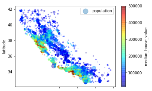
地理数据可视化
housing.plot(kind="scatter", x="longitude", y="latitude", alpha=0.4, s=housing["population"]/100, label="population",
 c="median_house_value", cmap=plt.get_cmap("jet"), colorbar=True,)
# 每个圈的半径表示街区的人口(选项`s`),颜色代表价格(选项`c`)
plt.legend()
查找关联
相关系数1
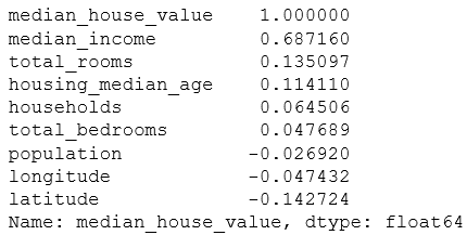
数据集不是很大时,可以很容易地使用corr()方法计算出每对属性间的标准相关系数(standard correlation coefficient,也称作皮尔逊相关系数)
corr_matrix = housing.corr()
corr_matrix["median_house_value"].sort_values(ascending=False)
相关系数2
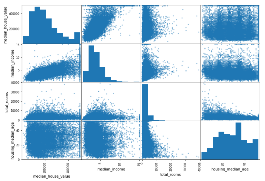
scatter_matrix函数,它能画出每个数值属性对每个其它数值属性的图。attributes = ["median_house_value", "median_income", "total_rooms", "housing_median_age"] pd.plotting.scatter_matrix(housing[attributes], figsize=(12, 8))
属性组合实验
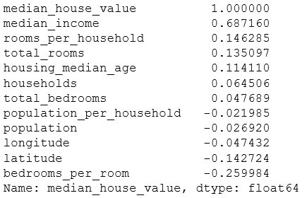
某些属性本身没有用,与其它属性结合起来就有用了。比如下面房间数与房主数本身没有用,相除得出的每户的房间数更有用。所以实际操作中需要各种属性组合,然后比较相关系数。
housing["rooms_per_household"] = housing["total_rooms"]/housing["households"]
housing["bedrooms_per_room"] = housing["total_bedrooms"]/housing["total_rooms"]
housing["population_per_household"]=housing["population"]/housing["households"]

corr_matrix = housing.corr()
corr_matrix["median_house_value"].sort_values(ascending=False)
不要手工来做,需要一些函数。原因:
- 函数可以在任何数据集上方便重复地数据转换
- 慢慢建立一个函数库,在未来的项目中重复使用
- 可以方便尝试多种数据转换
第一步,将特征和标签分开
housing = strat_train_set.drop("median_house_value", axis=1)
housing_labels = strat_train_set["median_house_value"]
数据清洗
缺失值(本例使用total_bedrooms):
- 去掉对应的街区
dropna() - 去掉整个属性
drop() - 进行赋值(0,平均值,中位数等)
fillna()使用该方法时记得保存平均值或者中位值等,后面测试集也要填充
housing.dropna(subset=["total_bedrooms"])  # 选项1
housing.drop("total_bedrooms", axis=1) # 选项2
median = housing["total_bedrooms"].median()
housing["total_bedrooms"].fillna(median) # 选项3
scikit-learn提供了一个类来处理缺失值:Imputer
from sklearn.preprocessing import Imputer

imputer = Imputer(strategy="median")

# 因为只有数值属性才能算出中位数,我们需要创建一份不包括文本属性`ocean_proximity`的数据副本
housing_num = housing.drop("ocean_proximity", axis=1)

# 用`fit()`方法将`imputer`实例拟合到训练数据
imputer.fit(housing_num)
X = imputer.transform(housing_num)
housing_tr = pd.DataFrame(X, columns=housing_num.columns)
Scikit-Learn 设计
Scikit-Learn 设计的 API 设计的非常好。它的主要设计原则是:
-
一致性:所有对象的接口一致且简单:
- 估计器(estimator)。任何可以基于数据集对一些参数进行估计的对象都被称为估计器(比如,
imputer就是个估计器)。估计本身是通过fit()方法,只需要一个数据集作为参数(对于监督学习算法,需要两个数据集;第二个数据集包含标签)。任何其它用来指导估计过程的参数都被当做超参数(比如imputer的strategy),并且超参数要被设置成实例变量(通常通过构造器参数设置)。 - 转换器(transformer)。一些估计器(比如
imputer)也可以转换数据集,这些估计器被称为转换器。API也是相当简单:转换是通过transform()方法,被转换的数据集作为参数。返回的是经过转换的数据集。转换过程依赖学习到的参数,比如imputer的例子。所有的转换都有一个便捷的方法fit_transform(),等同于调用fit()再transform()(但有时fit_transform()经过优化,运行的更快)。 - 预测器(predictor)。最后,一些估计器可以根据给出的数据集做预测,这些估计器称为预测器。例如,上一章的
LinearRegression模型就是一个预测器:它根据一个国家的人均 GDP 预测生活满意度。预测器有一个predict()方法,可以用新实例的数据集做出相应的预测。预测器还有一个score()方法,可用于评估测试集(如果是监督学习算法的话,还要给出相应的标签)的预测质量。
- 估计器(estimator)。任何可以基于数据集对一些参数进行估计的对象都被称为估计器(比如,
-
可检验。所有估计器的超参数都可以通过实例的public变量直接访问(比如,
imputer.strategy),并且所有估计器学习到的参数也可以通过在实例变量名后加下划线来访问(比如,imputer.statistics_)。 -
类不可扩散。数据集被表示成 NumPy 数组或 SciPy 稀疏矩阵,而不是自制的类。超参数只是普通的 Python 字符串或数字。
-
可组合。尽可能使用现存的模块。例如,用任意的转换器序列加上一个估计器,就可以做成一个流水线,后面会看到例子。
-
合理的默认值。Scikit-Learn 给大多数参数提供了合理的默认值,很容易就能创建一个系统。
处理文本和类别属性
from sklearn.preprocessing import LabelEncoder

encoder = LabelEncoder()
housing_cat = housing["ocean_proximity"]
housing_cat_encoded = encoder.fit_transform(housing_cat)
housing_cat_encoded
OneHotEncoder
原理是创建一个二元属性,当分类是<1H OCEAN,该属性为 1(否则为 0),当分类是INLAND,另一个属性等于 1(否则为 0),以此类推。这称作独热编码(One-Hot Encoding),因为只有一个属性会等于 1(热),其余会是 0(冷)
注意:fit_transform()
用于 2D 数组,而housing_cat_encoded`是一个 1D 数组,所以需要将其变形
from sklearn.preprocessing import OneHotEncoder

encoder = OneHotEncoder()
housing_cat_1hot = encoder.fit_transform(housing_cat_encoded.reshape(-1,1))
# housing_cat_1hot结果是一个稀疏矩阵,即只存储非零项。这是为了当分类很多时节省内存。 将其转换成numpy数组需要用到toarray函数
housing_cat_1hot.toarray()

LabelBinarizer
使用类LabelBinarizer,可以用一步执行这两个转换(从文本分类到整数分类,再从整数分类到独热向量)
from sklearn.preprocessing import LabelBinarizer

encoder = LabelBinarizer()
housing_cat_1hot = encoder.fit_transform(housing_cat)
housing_cat_1hot
注意默认返回的结果是一个密集 NumPy 数组。向构造器LabelBinarizer传递sparse_output=True,就可以得到一个稀疏矩阵。
自定义转换器
尽管 Scikit-Learn 提供了许多有用的转换器,你还是需要自己动手写转换器执行任务,比如自定义的清理操作,或属性组合。你需要让自制的转换器与 Scikit-Learn 组件(比如流水线)无缝衔接工作,因为 Scikit-Learn 是依赖鸭子类型的(而不是继承),你所需要做的是创建一个类并执行三个方法:fit()(返回self),transform(),和fit_transform()。通过添加TransformerMixin作为基类,可以很容易地得到最后一个。另外,如果你添加BaseEstimator作为基类(且构造器中避免使用*args和**kargs),你就能得到两个额外的方法(get_params()和set_params()),二者可以方便地进行超参数自动微调。例如,一个小转换器类添加了上面讨论的属性:
from sklearn.base import BaseEstimator, TransformerMixin
rooms_ix, bedrooms_ix, population_ix, household_ix = 3, 4, 5, 6

class CombinedAttributesAdder(BaseEstimator, TransformerMixin):
  def __init__(self, add_bedrooms_per_room = True): # no *args or **kargs
    self.add_bedrooms_per_room = add_bedrooms_per_room
  def fit(self, X, y=None):
    return self # nothing else to do
  def transform(self, X, y=None):
    rooms_per_household = X[:, rooms_ix] / X[:, household_ix]
    population_per_household = X[:, population_ix] / X[:, household_ix]
    if self.add_bedrooms_per_room:
      bedrooms_per_room = X[:, bedrooms_ix] / X[:, rooms_ix]
      return np.c_[X, rooms_per_household, population_per_household,
  bedrooms_per_room]
    else:
      return np.c_[X, rooms_per_household, population_per_household]

attr_adder = CombinedAttributesAdder(add_bedrooms_per_room=False)
housing_extra_attribs = attr_adder.transform(housing.values)
特征缩放
属性的量度相差很大时,模型性能会很差。比如某个属性范围是0-1,另外一个属性的值是10000-50000.这种情况就需要进行特征缩放。有两种方法:
- 线性函数归一化:cikit-Learn 提供了一个转换器
MinMaxScaler来实现这个功能。 - 标准化:Scikit-Learn 提供了一个转换器
StandardScaler来进行标准化。警告:缩放器只用于训练集拟合。
转换流水线
由上可以看出,很多转换步骤需要按照一定的数据。Scikit-Learn 提供了类Pipeline,来进行这一系列的转换。
只对数值的流水线
from sklearn.pipeline import Pipeline
from sklearn.preprocessing import StandardScaler

num_pipeline = Pipeline([
 ('imputer', Imputer(strategy="median")),
 ('attribs_adder', CombinedAttributesAdder()),
 ('std_scaler', StandardScaler()),
 ])
housing_num_tr = num_pipeline.fit_transform(housing_num)
scikit-learn中没有工具来处理Pandas的DataFrame,所以我们需要来写一个简单的自定义转换器来做这项工作
from sklearn.base import BaseEstimator, TransformerMixin

class DataFrameSelector(BaseEstimator, TransformerMixin):
  def __init__(self, attribute_names):
    self.attribute_names = attribute_names
  def fit(self, X, y=None):
    return self
  def transform(self, X):
    return X[self.attribute_names].values
一个完整的处理数值以及类别属性的流水线
# 由于sklearn更新使得LabelBinarizer的fit_transform只能接受两个参数,直接运行的话会报错,所以重写一个转化器,增加一个参数。
from sklearn.base import TransformerMixin #gives fit_transform method for free
class MyLabelBinarizer(TransformerMixin):
    def __init__(self, *args, **kwargs):
        self.encoder = LabelBinarizer(*args, **kwargs)
    def fit(self, x, y=0):
        self.encoder.fit(x)
        return self
    def transform(self, x, y=0):
        return self.encoder.transform(x)
from sklearn.pipeline import FeatureUnion

num_attribs = list(housing_num)
cat_attribs = ["ocean_proximity"]

num_pipeline = Pipeline([
 ('selector', DataFrameSelector(num_attribs)),
 ('imputer', Imputer(strategy="median")),
 ('attribs_adder', CombinedAttributesAdder()),
 ('std_scaler', StandardScaler()),
 ])

cat_pipeline = Pipeline([
 ('selector', DataFrameSelector(cat_attribs)),
 ('Mylabel_binarizer', MyLabelBinarizer()),
 ])

full_pipeline = FeatureUnion(transformer_list=[
 ("num_pipeline", num_pipeline),
 ("cat_pipeline", cat_pipeline),
 ])
housing_prepared = full_pipeline.fit_transform(housing)
housing_prepared[0]
选择并训练模型
线性模型使用与评估
from sklearn.linear_model import LinearRegression

lin_reg = LinearRegression()
lin_reg.fit(housing_prepared, housing_labels)

#结果0.6558010255907188
评估方式1:RMSE
用mean_squared_error`函数计算一下RMSE(欧几里得范数的平方根的和的根)
结果68628万美元的误差显然不能让人满意,欠拟合
from sklearn.metrics import mean_squared_error

housing_predictions = lin_reg.predict(housing_prepared)
lin_mse = mean_squared_error(housing_labels, housing_predictions)
lin_rmse = np.sqrt(lin_mse)
lin_rmse
评估方式2:交叉验证法
将数据集分成k个大小相似的互斥子集,每个子集保持数据分布的一致。然后,每次用k-1个子集的并集作为训练集,剩下的一个作为测试集,最终返回k个测试结果的均值。k最长用的取值是10,另外5和20也比较常用。
from sklearn.model_selection import cross_val_score

lin_scores = cross_val_score(lin_reg, housing_prepared, housing_labels,scoring="neg_mean_squared_error", cv=10)
lin_rmse_scores = np.sqrt(-lin_scores)

# lin_scores越大越好,取负值开方后的lin_rmse_scores越小越好
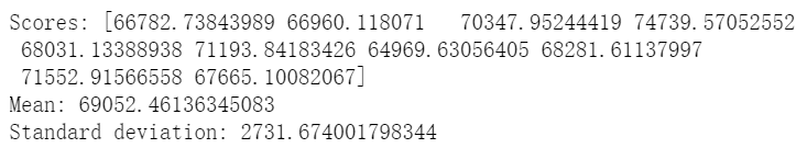
def display_scores(scores):
    print("Scores:", scores)
    print("Mean:", scores.mean())
    print("Standard deviation:", scores.std())
display_scores(lin_rmse_scores)
# Mean就是RMSE
决策树
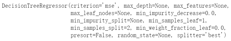
也可以换其它的模型试试,下面换DecisionTreeRegressor模型
from sklearn.tree import DecisionTreeRegressor

tree_reg = DecisionTreeRegressor()
tree_reg.fit(housing_prepared, housing_labels)
评估方式1:RMSE
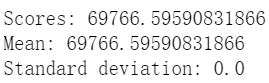
housing_predictions = tree_reg.predict(housing_prepared)
tree_mse = mean_squared_error(housing_labels, housing_predictions)
tree_rmse = np.sqrt(tree_mse)
tree_rmse
#结果 0.0
评估方式2:交叉验证
scores = cross_val_score(tree_reg, housing_prepared, housing_labels, scoring="neg_mean_squared_error", cv=10)
tree_rmse_scores = np.sqrt(-scores)

display_scores(tree_rmse_scores)

随机森林
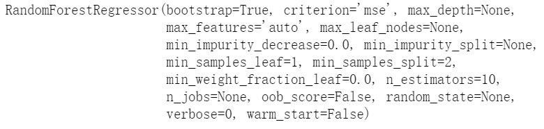
RandomForestRegressor
from sklearn.ensemble import RandomForestRegressor

forest_reg = RandomForestRegressor()
forest_reg.fit(housing_prepared, housing_labels)
评估方式1:RMSE
housing_predictions = forest_reg.predict(housing_prepared)
forest_mse = mean_squared_error(housing_labels, housing_predictions)
forest_rmse = np.sqrt(forest_mse)
forest_rmse
#22088.901578494966
评估方式2:交叉验证
scores = cross_val_score(forest_reg, housing_prepared, housing_labels, scoring="neg_mean_squared_error", cv=10)
forest_rmse_scores = np.sqrt(-scores)

display_scores(forest_rmse_scores)

比较下来,随机森林的评分52779.8955803107最小,性能最好,但是仍旧不够好。还需要给模型加一些限制,或者更多地训练数据来提高准确率。
模型微调
找到三五个还不错的模型,列成一个列表,然后对它们进行微调
网格搜索
微调就是手动调整超参数,但是做起来会非常繁杂。应该用Scikit-Learn 的GridSearchCV来做这项搜索工作
你所需要做的是告诉GridSearchCV要试验有哪些超参数,要试验什么值,GridSearchCV就能用交叉验证试验所有可能超参数值的组合。
from sklearn.model_selection import GridSearchCV

param_grid = [
 {'n_estimators': [3, 10, 30], 'max_features': [2, 4, 6, 8]},
 {'bootstrap': [False], 'n_estimators': [3, 10], 'max_features': [2, 3, 4]},
 ]

forest_reg = RandomForestRegressor()

grid_search = GridSearchCV(forest_reg, param_grid, cv=5, scoring='neg_mean_squared_error')
grid_search.fit(housing_prepared, housing_labels)
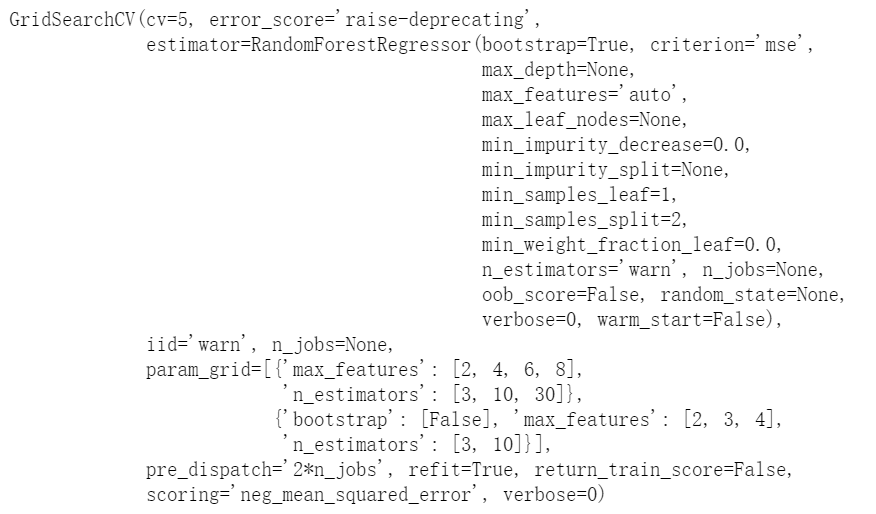
grid_search.best_params_
![]()
提示:因为 30 是n_estimators的最大值,你也应该估计更高的值,因为评估的分数可能会随n_estimators的增大而持续提升。
你还能直接得到最佳的估计器:
grid_search.best_estimator_

# 得到评估得分
cvres = grid_search.cv_results_
for mean_score, params in zip(cvres["mean_test_score"], cvres["params"]):
    print(np.sqrt(-mean_score), params)

通过网格搜索,找到'max_features': 8, 'n_estimators': 30下的RMSE为49897,低于全部默认值时的52779。微调成功
随机搜索
搜索组合较多时,网格搜索就不太适用了。这时最好使用RandomizedSearchCV
它不是尝试所有可能的组合,而是通过选择每个超参数的一个随机值的特定数量的随机组合。
集成方法
另一种微调系统的方法是将表现最好的模型组合起来。组合(集成)之后的性能通常要比单独的模型要好
分析最佳模型和它们的误差
可以指出每个属性对于做出准确预测的相对重要性
feature_importances = grid_search.best_estimator_.feature_importances_
feature_importances
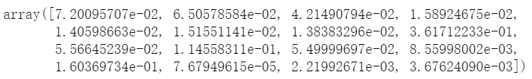
将重要性分数和属性名放到一起
extra_attribs = ["rooms_per_hhold", "pop_per_hhold", "bedrooms_per_room"]

cat_one_hot_attribs = list(encoder.classes_)
attributes = num_attribs + extra_attribs + cat_one_hot_attribs

sorted(zip(feature_importances,attributes), reverse=True)
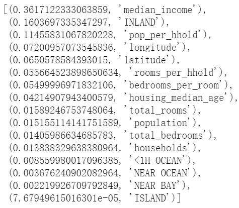
由上可以看出,字段中ISLAND最重要,其它的几个可以删掉
用测试集评估系统
final_model = grid_search.best_estimator_

X_test = strat_test_set.drop("median_house_value", axis=1)
y_test = strat_test_set["median_house_value"].copy()
X_test_prepared = full_pipeline.transform(X_test)

final_predictions = final_model.predict(X_test_prepared)

final_mse = mean_squared_error(y_test, final_predictions)
final_rmse = np.sqrt(final_mse)

display_scores(final_rmse)
启动、监控、维护系统
你还需要编写监控代码,以固定间隔检测系统的实时表现,当发生下降时触发报警。这对于捕获突然的系统崩溃和性能下降十分重要。做监控很常见,是因为模型会随着数据的演化而性能下降,除非模型用新数据定期训练。
评估系统的表现需要对预测值采样并进行评估。这通常需要人来分析。分析者可能是领域专家,或者是众包平台(比如 Amazon Mechanical Turk 或 CrowdFlower)的工人。不管采用哪种方法,你都需要将人工评估的流水线植入系统。
你还要评估系统输入数据的质量。有时因为低质量的信号(比如失灵的传感器发送随机值,或另一个团队的输出停滞),系统的表现会逐渐变差,但可能需要一段时间,系统的表现才能下降到一定程度,触发警报。如果监测了系统的输入,你就可能尽量早的发现问题。对于线上学习系统,监测输入数据是非常重要的。
最后,你可能想定期用新数据训练模型。你应该尽可能自动化这个过程。如果不这么做,非常有可能你需要每隔至少六个月更新模型,系统的表现就会产生严重波动。如果你的系统是一个线上学习系统,你需要定期保存系统状态快照,好能方便地回滚到之前的工作状态。