Background
Latest Data Source: https://www.ssa.gov/oact/babynames/limits.html
yobYYYY.txt (1880 ~ 2016)
name,sex,number
这是一个非常标准的以逗号隔开的格式,可以用pandas.read_csv将其加载到DataFrame中。
 1 C:UsersI******>ipython --pylab
 2 Python 2.7.13 | 64-bit | (default, Mar 30 2017, 11:20:05) [MSC v.1500 64 bit (AMD64)]
 3 Type "copyright", "credits" or "license" for more information.
 4
 5 IPython 4.1.2 -- An enhanced Interactive Python.
 6 ?         -> Introduction and overview of IPython's features.
 7 %quickref -> Quick reference.
 8 help      -> Python's own help system.
 9 object?   -> Details about 'object', use 'object??' for extra details.
10 Using matplotlib backend: TkAgg
11
12 In [1]: import pandas as pd
13
14 In [2]: names1880 = pd.read_csv('C:/Users/I******/Desktop/.../names/yob1880.txt', names=['name', 'sex', 'number'])
15
16 In [3]: names1880
17 Out[3]:
18            name sex  number
19 0          Mary   F    7065
20 1          Anna   F    2604
21 2          Emma   F    2003
22 3     Elizabeth   F    1939
23 4        Minnie   F    1746
24 5      Margaret   F    1578
25 6           Ida   F    1472
26 7         Alice   F    1414
27 8        Bertha   F    1320
28 9         Sarah   F    1288
29 10        Annie   F    1258
30 11        Clara   F    1226
31 12         Ella   F    1156
32 13     Florence   F    1063
33 14         Cora   F    1045
34 15       Martha   F    1040
35 16        Laura   F    1012
36 17       Nellie   F     995
37 18        Grace   F     982
38 19       Carrie   F     949
39 20        Maude   F     858
40 21        Mabel   F     808
41 22       Bessie   F     796
42 23       Jennie   F     793
43 24     Gertrude   F     787
44 25        Julia   F     783
45 26       Hattie   F     769
46 27        Edith   F     768
47 28       Mattie   F     704
48 29         Rose   F     700
49 ...         ...  ..     ...
50 1970      Philo   M       5
51 1971    Phineas   M       5
52 1972    Presley   M       5
53 1973     Ransom   M       5
54 1974      Reece   M       5
55 1975       Rene   M       5
56 1976    Roswell   M       5
57 1977    Rowland   M       5
58 1978    Sampson   M       5
59 1979     Samual   M       5
60 1980     Santos   M       5
61 1981   Schuyler   M       5
62 1982   Sheppard   M       5
63 1983   Spurgeon   M       5
64 1984   Starling   M       5
65 1985   Sylvanus   M       5
66 1986   Theadore   M       5
67 1987  Theophile   M       5
68 1988     Tilmon   M       5
69 1989      Tommy   M       5
70 1990    Unknown   M       5
71 1991       Vann   M       5
72 1992        Wes   M       5
73 1993    Winston   M       5
74 1994       Wood   M       5
75 1995     Woodie   M       5
76 1996     Worthy   M       5
77 1997     Wright   M       5
78 1998       York   M       5
79 1999  Zachariah   M       5
80
81 [2000 rows x 3 columns]
用number列的sex分组小计表示该年度的number总计。
1 In [4]: names1880.groupby('sex').number.sum()
2 Out[4]:
3 sex
4 F     90992
5 M    110491
6 Name: number, dtype: int64
将所有数据组装到一个DataFrame里面,并加上一个year字段。使用pandas.concat即可达到这个目的。
注意:第一,concat默认是按行将多个DataFrame组合到一起的;第二,必须指定ignore_index=True,因为我们不希望保留read_csv所返回的原始行号。
 1 In [5]: years = range(1880, 2017)
 2
 3 In [6]: pieces = []
 4
 5 In [7]: columns = ['name', 'sex', 'number']
 6
 7 In [8]: for year in years:
 8    ...:     path = 'C:/Users/I******/Desktop/.../names/yob%d.txt' % year
 9    ...:     frame = pd.read_csv(path, names=columns)
10    ...:     frame['year'] = year
11    ...:     pieces.append(frame)
12    ...:
13
14 In [9]: names = pd.concat(pieces, ignore_index=True)
15
16 In [10]: names
17 Out[10]:
18               name sex  number  year
19 0             Mary   F    7065  1880
20 1             Anna   F    2604  1880
21 2             Emma   F    2003  1880
22 3        Elizabeth   F    1939  1880
23 4           Minnie   F    1746  1880
24 5         Margaret   F    1578  1880
25 6              Ida   F    1472  1880
26 7            Alice   F    1414  1880
27 8           Bertha   F    1320  1880
28 9            Sarah   F    1288  1880
29 10           Annie   F    1258  1880
30 11           Clara   F    1226  1880
31 12            Ella   F    1156  1880
32 13        Florence   F    1063  1880
33 14            Cora   F    1045  1880
34 15          Martha   F    1040  1880
35 16           Laura   F    1012  1880
36 17          Nellie   F     995  1880
37 18           Grace   F     982  1880
38 19          Carrie   F     949  1880
39 20           Maude   F     858  1880
40 21           Mabel   F     808  1880
41 22          Bessie   F     796  1880
42 23          Jennie   F     793  1880
43 24        Gertrude   F     787  1880
44 25           Julia   F     783  1880
45 26          Hattie   F     769  1880
46 27           Edith   F     768  1880
47 28          Mattie   F     704  1880
48 29            Rose   F     700  1880
49 ...            ...  ..     ...   ...
50 1891864    Zariyan   M       5  2016
51 1891865     Zarren   M       5  2016
52 1891866      Zaryn   M       5  2016
53 1891867      Zaxon   M       5  2016
54 1891868     Zaxtyn   M       5  2016
55 1891869       Zaye   M       5  2016
56 1891870     Zaymar   M       5  2016
57 1891871     Zaymir   M       5  2016
58 1891872      Zaynn   M       5  2016
59 1891873   Zayshaun   M       5  2016
60 1891874     Zedric   M       5  2016
61 1891875   Zekariah   M       5  2016
62 1891876      Zelan   M       5  2016
63 1891877     Zephen   M       5  2016
64 1891878   Zephyrus   M       5  2016
65 1891879      Zeric   M       5  2016
66 1891880      Zerin   M       5  2016
67 1891881     Zethan   M       5  2016
68 1891882      Zihao   M       5  2016
69 1891883       Zimo   M       5  2016
70 1891884       Zinn   M       5  2016
71 1891885      Zirui   M       5  2016
72 1891886       Ziya   M       5  2016
73 1891887     Ziyang   M       5  2016
74 1891888       Zoel   M       5  2016
75 1891889     Zolton   M       5  2016
76 1891890     Zurich   M       5  2016
77 1891891     Zyahir   M       5  2016
78 1891892       Zyel   M       5  2016
79 1891893      Zylyn   M       5  2016
80
81 [1891894 rows x 4 columns]
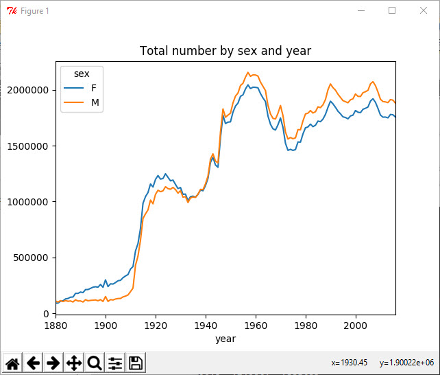
按年份、性别计数。
 1 In [11]: total_number = names.pivot_table('number', index='year', columns='sex', aggfunc=sum)
 2
 3 In [12]: total_number.tail()
 4 Out[12]:
 5 sex         F        M
 6 year
 7 2012  1756347  1892094
 8 2013  1749061  1885683
 9 2014  1779496  1913434
10 2015  1776538  1907211
11 2016  1756647  1880674
作图。
1 In [13]: total_number.plot(title='Total number by sex and year')
插入一个prop列,用于存放指定名字的婴儿数相对于总出生数的比例。
 1 In [14]: def add_prop(group):
 2    ....:     number = group.number.astype(float)
 3    ....:     group['prop'] = number / number.sum()
 4    ....:     return group
 5    ....:
 6
 7 In [15]: names = names.groupby(['year', 'sex']).apply(add_prop)
 8
 9 In [16]: names
10 Out[16]:
11               name sex  number  year      prop
12 0             Mary   F    7065  1880  0.077644
13 1             Anna   F    2604  1880  0.028618
14 2             Emma   F    2003  1880  0.022013
15 3        Elizabeth   F    1939  1880  0.021310
16 4           Minnie   F    1746  1880  0.019189
17 5         Margaret   F    1578  1880  0.017342
18 6              Ida   F    1472  1880  0.016177
19 7            Alice   F    1414  1880  0.015540
20 8           Bertha   F    1320  1880  0.014507
21 9            Sarah   F    1288  1880  0.014155
22 10           Annie   F    1258  1880  0.013825
23 11           Clara   F    1226  1880  0.013474
24 12            Ella   F    1156  1880  0.012704
25 13        Florence   F    1063  1880  0.011682
26 14            Cora   F    1045  1880  0.011485
27 15          Martha   F    1040  1880  0.011430
28 16           Laura   F    1012  1880  0.011122
29 17          Nellie   F     995  1880  0.010935
30 18           Grace   F     982  1880  0.010792
31 19          Carrie   F     949  1880  0.010429
32 20           Maude   F     858  1880  0.009429
33 21           Mabel   F     808  1880  0.008880
34 22          Bessie   F     796  1880  0.008748
35 23          Jennie   F     793  1880  0.008715
36 24        Gertrude   F     787  1880  0.008649
37 25           Julia   F     783  1880  0.008605
38 26          Hattie   F     769  1880  0.008451
39 27           Edith   F     768  1880  0.008440
40 28          Mattie   F     704  1880  0.007737
41 29            Rose   F     700  1880  0.007693
42 ...            ...  ..     ...   ...       ...
43 1891864    Zariyan   M       5  2016  0.000003
44 1891865     Zarren   M       5  2016  0.000003
45 1891866      Zaryn   M       5  2016  0.000003
46 1891867      Zaxon   M       5  2016  0.000003
47 1891868     Zaxtyn   M       5  2016  0.000003
48 1891869       Zaye   M       5  2016  0.000003
49 1891870     Zaymar   M       5  2016  0.000003
50 1891871     Zaymir   M       5  2016  0.000003
51 1891872      Zaynn   M       5  2016  0.000003
52 1891873   Zayshaun   M       5  2016  0.000003
53 1891874     Zedric   M       5  2016  0.000003
54 1891875   Zekariah   M       5  2016  0.000003
55 1891876      Zelan   M       5  2016  0.000003
56 1891877     Zephen   M       5  2016  0.000003
57 1891878   Zephyrus   M       5  2016  0.000003
58 1891879      Zeric   M       5  2016  0.000003
59 1891880      Zerin   M       5  2016  0.000003
60 1891881     Zethan   M       5  2016  0.000003
61 1891882      Zihao   M       5  2016  0.000003
62 1891883       Zimo   M       5  2016  0.000003
63 1891884       Zinn   M       5  2016  0.000003
64 1891885      Zirui   M       5  2016  0.000003
65 1891886       Ziya   M       5  2016  0.000003
66 1891887     Ziyang   M       5  2016  0.000003
67 1891888       Zoel   M       5  2016  0.000003
68 1891889     Zolton   M       5  2016  0.000003
69 1891890     Zurich   M       5  2016  0.000003
70 1891891     Zyahir   M       5  2016  0.000003
71 1891892       Zyel   M       5  2016  0.000003
72 1891893      Zylyn   M       5  2016  0.000003
73
74 [1891894 rows x 5 columns]
注意:整数除法会向下圆整,由于number是整数,所以在计算分式时必须将分子或分母转换成浮点数。
在执行这样的分组处理时,一般都应该做一些有效性检查,比如验证所有分组的prop的总和是否为1。由于这是一个浮点型数据,所以用np.allclose来检查这个分组的总计值是否足够近似于(可能不会精确等于)1。
1 In [17]: np.allclose(names.groupby(['year', 'sex']).prop.sum(), 1)
2 Out[17]: True
为了便于实现更进一步的分析,取出该数据的一个子集:每对sex/year组合的前1000个名字。这又是一个分组操作。
 1 In [18]: def get_top1000(group):
 2    ....:     return group.sort_values(by='number', ascending=False)[:1000]
 3    ....:
 4
 5 In [19]: grouped = names.groupby(['year', 'sex'])
 6
 7 In [20: top1000 = grouped.apply(get_top1000)
 8
 9 In [21]: pieces = []
10
11 In [22]: for year, group in names.groupby(['year', 'sex']):
12    ....:     pieces.append(group.sort_values(by='number', ascending=False)[:1000])
13    ....:
14
15 In [23]: top1000 = pd.concat(pieces, ignore_index=True)
16
17 In [24]: top1000
18 Out[24]:
19              name sex  number  year      prop
20 0            Mary   F    7065  1880  0.077644
21 1            Anna   F    2604  1880  0.028618
22 2            Emma   F    2003  1880  0.022013
23 3       Elizabeth   F    1939  1880  0.021310
24 4          Minnie   F    1746  1880  0.019189
25 5        Margaret   F    1578  1880  0.017342
26 6             Ida   F    1472  1880  0.016177
27 7           Alice   F    1414  1880  0.015540
28 8          Bertha   F    1320  1880  0.014507
29 9           Sarah   F    1288  1880  0.014155
30 10          Annie   F    1258  1880  0.013825
31 11          Clara   F    1226  1880  0.013474
32 12           Ella   F    1156  1880  0.012704
33 13       Florence   F    1063  1880  0.011682
34 14           Cora   F    1045  1880  0.011485
35 15         Martha   F    1040  1880  0.011430
36 16          Laura   F    1012  1880  0.011122
37 17         Nellie   F     995  1880  0.010935
38 18          Grace   F     982  1880  0.010792
39 19         Carrie   F     949  1880  0.010429
40 20          Maude   F     858  1880  0.009429
41 21          Mabel   F     808  1880  0.008880
42 22         Bessie   F     796  1880  0.008748
43 23         Jennie   F     793  1880  0.008715
44 24       Gertrude   F     787  1880  0.008649
45 25          Julia   F     783  1880  0.008605
46 26         Hattie   F     769  1880  0.008451
47 27          Edith   F     768  1880  0.008440
48 28         Mattie   F     704  1880  0.007737
49 29           Rose   F     700  1880  0.007693
50 ...           ...  ..     ...   ...       ...
51 273847      Keanu   M     210  2016  0.000112
52 273848     Konner   M     210  2016  0.000112
53 273849      Brent   M     209  2016  0.000111
54 273850   Immanuel   M     209  2016  0.000111
55 273851    Benicio   M     208  2016  0.000111
56 273852     Ernest   M     208  2016  0.000111
57 273853    Merrick   M     208  2016  0.000111
58 273854    Yisroel   M     208  2016  0.000111
59 273855       Lyle   M     207  2016  0.000110
60 273856      Amare   M     207  2016  0.000110
61 273857        Jad   M     207  2016  0.000110
62 273858     Maddux   M     206  2016  0.000110
63 273859      Creed   M     206  2016  0.000110
64 273860      Krish   M     206  2016  0.000110
65 273861  Giancarlo   M     205  2016  0.000109
66 273862   Jamarion   M     205  2016  0.000109
67 273863      Steve   M     205  2016  0.000109
68 273864     Camilo   M     205  2016  0.000109
69 273865      Anton   M     204  2016  0.000108
70 273866      Jamar   M     204  2016  0.000108
71 273867   Jeremias   M     204  2016  0.000108
72 273868      Ralph   M     204  2016  0.000108
73 273869     Wesson   M     204  2016  0.000108
74 273870    Brenden   M     203  2016  0.000108
75 273871    Eliezer   M     203  2016  0.000108
76 273872    Braeden   M     203  2016  0.000108
77 273873       Bode   M     203  2016  0.000108
78 273874     Davian   M     202  2016  0.000107
79 273875        Gus   M     202  2016  0.000107
80 273876   Jonathon   M     202  2016  0.000107
81
82 [273877 rows x 5 columns]
分析命名趋势。
首先将前1000个名字分为男女两个部分。
1 In [25]: boys = top1000[top1000.sex == 'M']
2
3 In [26]: girls = top1000[top1000.sex == 'F']
生成一张按year和name统计的总出生数透视表。
  1 In [27]: total_number = top1000.pivot_table('number', index='year', columns='name', aggfunc=sum)
  2
  3 In [28]: total_number
  4 Out[28]:
  5 name   Aaden  Aadhya  Aaliyah  Aanya  Aarav    Aaron  Aarush   Ab  Abagail
  6 year
  7 1880     NaN     NaN      NaN    NaN    NaN    102.0     NaN  NaN      NaN
  8 1881     NaN     NaN      NaN    NaN    NaN     94.0     NaN  NaN      NaN
  9 1882     NaN     NaN      NaN    NaN    NaN     85.0     NaN  NaN      NaN
 10 1883     NaN     NaN      NaN    NaN    NaN    105.0     NaN  NaN      NaN
 11 1884     NaN     NaN      NaN    NaN    NaN     97.0     NaN  NaN      NaN
 12 1885     NaN     NaN      NaN    NaN    NaN     88.0     NaN  6.0      NaN
 13 1886     NaN     NaN      NaN    NaN    NaN     86.0     NaN  NaN      NaN
 14 1887     NaN     NaN      NaN    NaN    NaN     78.0     NaN  NaN      NaN
 15 1888     NaN     NaN      NaN    NaN    NaN     90.0     NaN  NaN      NaN
 16 1889     NaN     NaN      NaN    NaN    NaN     85.0     NaN  NaN      NaN
 17 1890     NaN     NaN      NaN    NaN    NaN     96.0     NaN  NaN      NaN
 18 1891     NaN     NaN      NaN    NaN    NaN     69.0     NaN  NaN      NaN
 19 1892     NaN     NaN      NaN    NaN    NaN     95.0     NaN  NaN      NaN
 20 1893     NaN     NaN      NaN    NaN    NaN     81.0     NaN  NaN      NaN
 21 1894     NaN     NaN      NaN    NaN    NaN     79.0     NaN  NaN      NaN
 22 1895     NaN     NaN      NaN    NaN    NaN     94.0     NaN  NaN      NaN
 23 1896     NaN     NaN      NaN    NaN    NaN     69.0     NaN  NaN      NaN
 24 1897     NaN     NaN      NaN    NaN    NaN     87.0     NaN  NaN      NaN
 25 1898     NaN     NaN      NaN    NaN    NaN     89.0     NaN  NaN      NaN
 26 1899     NaN     NaN      NaN    NaN    NaN     71.0     NaN  NaN      NaN
 27 1900     NaN     NaN      NaN    NaN    NaN    103.0     NaN  NaN      NaN
 28 1901     NaN     NaN      NaN    NaN    NaN     80.0     NaN  NaN      NaN
 29 1902     NaN     NaN      NaN    NaN    NaN     78.0     NaN  NaN      NaN
 30 1903     NaN     NaN      NaN    NaN    NaN     93.0     NaN  NaN      NaN
 31 1904     NaN     NaN      NaN    NaN    NaN    117.0     NaN  NaN      NaN
 32 1905     NaN     NaN      NaN    NaN    NaN     96.0     NaN  NaN      NaN
 33 1906     NaN     NaN      NaN    NaN    NaN     96.0     NaN  NaN      NaN
 34 1907     NaN     NaN      NaN    NaN    NaN    130.0     NaN  NaN      NaN
 35 1908     NaN     NaN      NaN    NaN    NaN    114.0     NaN  NaN      NaN
 36 1909     NaN     NaN      NaN    NaN    NaN    142.0     NaN  NaN      NaN
 37 ...      ...     ...      ...    ...    ...      ...     ...  ...      ...
 38 1987     NaN     NaN      NaN    NaN    NaN  12682.0     NaN  NaN      NaN
 39 1988     NaN     NaN      NaN    NaN    NaN  14404.0     NaN  NaN      NaN
 40 1989     NaN     NaN      NaN    NaN    NaN  15312.0     NaN  NaN      NaN
 41 1990     NaN     NaN      NaN    NaN    NaN  14550.0     NaN  NaN      NaN
 42 1991     NaN     NaN      NaN    NaN    NaN  14241.0     NaN  NaN      NaN
 43 1992     NaN     NaN      NaN    NaN    NaN  14506.0     NaN  NaN      NaN
 44 1993     NaN     NaN      NaN    NaN    NaN  13827.0     NaN  NaN      NaN
 45 1994     NaN     NaN   1451.0    NaN    NaN  14381.0     NaN  NaN      NaN
 46 1995     NaN     NaN   1255.0    NaN    NaN  13287.0     NaN  NaN      NaN
 47 1996     NaN     NaN    831.0    NaN    NaN  11969.0     NaN  NaN      NaN
 48 1997     NaN     NaN   1738.0    NaN    NaN  11165.0     NaN  NaN      NaN
 49 1998     NaN     NaN   1399.0    NaN    NaN  10547.0     NaN  NaN      NaN
 50 1999     NaN     NaN   1088.0    NaN    NaN   9853.0     NaN  NaN    211.0
 51 2000     NaN     NaN   1496.0    NaN    NaN   9551.0     NaN  NaN    222.0
 52 2001     NaN     NaN   3352.0    NaN    NaN   9534.0     NaN  NaN    244.0
 53 2002     NaN     NaN   4778.0    NaN    NaN   9001.0     NaN  NaN    256.0
 54 2003     NaN     NaN   3671.0    NaN    NaN   8862.0     NaN  NaN    276.0
 55 2004     NaN     NaN   3488.0    NaN    NaN   8388.0     NaN  NaN    258.0
 56 2005     NaN     NaN   3456.0    NaN    NaN   7800.0     NaN  NaN    288.0
 57 2006     NaN     NaN   3743.0    NaN    NaN   8294.0     NaN  NaN    298.0
 58 2007     NaN     NaN   3955.0    NaN    NaN   8933.0     NaN  NaN    313.0
 59 2008   956.0     NaN   4038.0    NaN  219.0   8536.0     NaN  NaN    321.0
 60 2009  1267.0     NaN   4367.0    NaN  270.0   7967.0     NaN  NaN    297.0
 61 2010   450.0     NaN   4661.0    NaN  438.0   7461.0   227.0  NaN    281.0
 62 2011   275.0     NaN   5112.0    NaN  436.0   7613.0     NaN  NaN      NaN
 63 2012   223.0     NaN   5502.0    NaN  435.0   7522.0     NaN  NaN      NaN
 64 2013   203.0     NaN   5225.0    NaN  495.0   7297.0     NaN  NaN      NaN
 65 2014   237.0     NaN   4875.0  266.0  531.0   7383.0     NaN  NaN      NaN
 66 2015   297.0     NaN   4850.0    NaN  539.0   7144.0   211.0  NaN      NaN
 67 2016     NaN   284.0   4611.0    NaN  519.0   7118.0     NaN  NaN      NaN
 68
 69 name  Abb   ...       Zoe    Zoey   Zoie  Zola  Zollie  Zona  Zora  Zula
 70 year        ...
 71 1880  NaN   ...      23.0     NaN    NaN   7.0     NaN   8.0  28.0  27.0
 72 1881  NaN   ...      22.0     NaN    NaN  10.0     NaN   9.0  21.0  27.0
 73 1882  NaN   ...      25.0     NaN    NaN   9.0     NaN  17.0  32.0  21.0
 74 1883  NaN   ...      23.0     NaN    NaN  10.0     NaN  11.0  35.0  25.0
 75 1884  NaN   ...      31.0     NaN    NaN  14.0     6.0   8.0  58.0  27.0
 76 1885  NaN   ...      27.0     NaN    NaN  12.0     6.0  14.0  48.0  38.0
 77 1886  NaN   ...      25.0     NaN    NaN   8.0     NaN  20.0  52.0  43.0
 78 1887  NaN   ...      34.0     NaN    NaN  23.0     NaN  28.0  46.0  33.0
 79 1888  NaN   ...      42.0     NaN    NaN  23.0     7.0  30.0  42.0  45.0
 80 1889  NaN   ...      29.0     NaN    NaN  22.0     NaN  29.0  53.0  55.0
 81 1890  6.0   ...      42.0     NaN    NaN  32.0     7.0  27.0  60.0  65.0
 82 1891  NaN   ...      34.0     NaN    NaN  29.0     6.0  14.0  52.0  45.0
 83 1892  NaN   ...      34.0     NaN    NaN  27.0     NaN  25.0  66.0  53.0
 84 1893  NaN   ...      23.0     NaN    NaN  34.0     6.0  15.0  67.0  70.0
 85 1894  NaN   ...      28.0     NaN    NaN  51.0     NaN  23.0  66.0  64.0
 86 1895  NaN   ...      34.0     NaN    NaN  60.0    11.0  38.0  55.0  55.0
 87 1896  NaN   ...      36.0     NaN    NaN  47.0     NaN  38.0  72.0  65.0
 88 1897  NaN   ...      35.0     NaN    NaN  51.0     NaN  28.0  67.0  79.0
 89 1898  NaN   ...      30.0     NaN    NaN  62.0     NaN  28.0  65.0  83.0
 90 1899  NaN   ...      27.0     NaN    NaN  49.0     6.0  31.0  56.0  60.0
 91 1900  NaN   ...      26.0     NaN    NaN  48.0     9.0  44.0  99.0  71.0
 92 1901  NaN   ...      26.0     NaN    NaN  56.0     NaN  31.0  58.0  57.0
 93 1902  NaN   ...      34.0     NaN    NaN  58.0     NaN  23.0  58.0  66.0
 94 1903  NaN   ...      19.0     NaN    NaN  64.0     NaN  41.0  83.0  74.0
 95 1904  NaN   ...      27.0     NaN    NaN  46.0     NaN  35.0  54.0  74.0
 96 1905  NaN   ...      24.0     NaN    NaN  66.0     8.0  24.0  55.0  61.0
 97 1906  NaN   ...      19.0     NaN    NaN  59.0     NaN  37.0  64.0  58.0
 98 1907  NaN   ...      19.0     NaN    NaN  53.0    11.0  39.0  92.0  72.0
 99 1908  NaN   ...      23.0     NaN    NaN  70.0     NaN  31.0  59.0  53.0
100 1909  NaN   ...      22.0     NaN    NaN  59.0     NaN  39.0  57.0  76.0
101 ...   ...   ...       ...     ...    ...   ...     ...   ...   ...   ...
102 1987  NaN   ...     247.0     NaN    NaN   NaN     NaN   NaN   NaN   NaN
103 1988  NaN   ...     241.0     NaN    NaN   NaN     NaN   NaN   NaN   NaN
104 1989  NaN   ...     376.0     NaN    NaN   NaN     NaN   NaN   NaN   NaN
105 1990  NaN   ...     478.0     NaN    NaN   NaN     NaN   NaN   NaN   NaN
106 1991  NaN   ...     722.0     NaN    NaN   NaN     NaN   NaN   NaN   NaN
107 1992  NaN   ...     981.0     NaN    NaN   NaN     NaN   NaN   NaN   NaN
108 1993  NaN   ...    1193.0     NaN    NaN   NaN     NaN   NaN   NaN   NaN
109 1994  NaN   ...    1333.0     NaN    NaN   NaN     NaN   NaN   NaN   NaN
110 1995  NaN   ...    1726.0   219.0    NaN   NaN     NaN   NaN   NaN   NaN
111 1996  NaN   ...    2065.0   339.0    NaN   NaN     NaN   NaN   NaN   NaN
112 1997  NaN   ...    2362.0   407.0    NaN   NaN     NaN   NaN   NaN   NaN
113 1998  NaN   ...    2693.0   478.0  225.0   NaN     NaN   NaN   NaN   NaN
114 1999  NaN   ...    3236.0   563.0  257.0   NaN     NaN   NaN   NaN   NaN
115 2000  NaN   ...    3785.0   691.0  320.0   NaN     NaN   NaN   NaN   NaN
116 2001  NaN   ...    4644.0   822.0  439.0   NaN     NaN   NaN   NaN   NaN
117 2002  NaN   ...    4886.0  1182.0  438.0   NaN     NaN   NaN   NaN   NaN
118 2003  NaN   ...    5085.0  1469.0  449.0   NaN     NaN   NaN   NaN   NaN
119 2004  NaN   ...    5363.0  1622.0  515.0   NaN     NaN   NaN   NaN   NaN
120 2005  NaN   ...    4958.0  2273.0  502.0   NaN     NaN   NaN   NaN   NaN
121 2006  NaN   ...    5152.0  2849.0  531.0   NaN     NaN   NaN   NaN   NaN
122 2007  NaN   ...    4933.0  3032.0  527.0   NaN     NaN   NaN   NaN   NaN
123 2008  NaN   ...    4781.0  3445.0  493.0   NaN     NaN   NaN   NaN   NaN
124 2009  NaN   ...    5144.0  3993.0  499.0   NaN     NaN   NaN   NaN   NaN
125 2010  NaN   ...    6264.0  5203.0  508.0   NaN     NaN   NaN   NaN   NaN
126 2011  NaN   ...    6299.0  6397.0  523.0   NaN     NaN   NaN   NaN   NaN
127 2012  NaN   ...    6451.0  7462.0  516.0   NaN     NaN   NaN   NaN   NaN
128 2013  NaN   ...    5969.0  7230.0  431.0   NaN     NaN   NaN   NaN   NaN
129 2014  NaN   ...    5866.0  7392.0  365.0   NaN     NaN   NaN   NaN   NaN
130 2015  NaN   ...    6032.0  6927.0  370.0   NaN     NaN   NaN   NaN   NaN
131 2016  NaN   ...    5706.0  6414.0  311.0   NaN     NaN   NaN   NaN   NaN
132
133 name   Zuri  Zyaire
134 year
135 1880    NaN     NaN
136 1881    NaN     NaN
137 1882    NaN     NaN
138 1883    NaN     NaN
139 1884    NaN     NaN
140 1885    NaN     NaN
141 1886    NaN     NaN
142 1887    NaN     NaN
143 1888    NaN     NaN
144 1889    NaN     NaN
145 1890    NaN     NaN
146 1891    NaN     NaN
147 1892    NaN     NaN
148 1893    NaN     NaN
149 1894    NaN     NaN
150 1895    NaN     NaN
151 1896    NaN     NaN
152 1897    NaN     NaN
153 1898    NaN     NaN
154 1899    NaN     NaN
155 1900    NaN     NaN
156 1901    NaN     NaN
157 1902    NaN     NaN
158 1903    NaN     NaN
159 1904    NaN     NaN
160 1905    NaN     NaN
161 1906    NaN     NaN
162 1907    NaN     NaN
163 1908    NaN     NaN
164 1909    NaN     NaN
165 ...     ...     ...
166 1987    NaN     NaN
167 1988    NaN     NaN
168 1989    NaN     NaN
169 1990    NaN     NaN
170 1991    NaN     NaN
171 1992    NaN     NaN
172 1993    NaN     NaN
173 1994    NaN     NaN
174 1995    NaN     NaN
175 1996    NaN     NaN
176 1997    NaN     NaN
177 1998    NaN     NaN
178 1999    NaN     NaN
179 2000    NaN     NaN
180 2001    NaN     NaN
181 2002    NaN     NaN
182 2003    NaN     NaN
183 2004    NaN     NaN
184 2005    NaN     NaN
185 2006    NaN     NaN
186 2007    NaN     NaN
187 2008    NaN     NaN
188 2009    NaN     NaN
189 2010  259.0     NaN
190 2011  313.0     NaN
191 2012  435.0     NaN
192 2013  567.0     NaN
193 2014  666.0     NaN
194 2015  712.0     NaN
195 2016  884.0   245.0
196
197 [137 rows x 7100 columns]
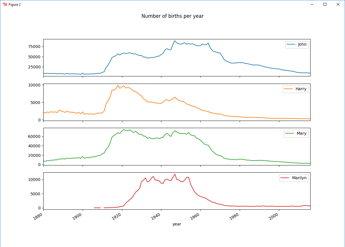
取出John、Harry、Mary和Marilyn这四个名字作为子集,并作图。
1 In [29]: subset = total_number[['John', 'Harry', 'Mary', 'Marilyn']]
2
3 In [30]: subset.plot(subplots=True, figsize=(12, 10), grid=False, title="Number of births per year")
评估命名多样性的增长
验证父母愿意给小孩起常见的名字越来越少:
一、计算最流行的1000个名字所占的比例,按year和sex进行聚合并绘图。
1 In [31]: table = top1000.pivot_table('prop', index='year', columns='sex', aggfunc=sum)
2
3 In [32]: table.plot(title='Sum of table1000.prop by year and sex', yticks=np.linspace(0, 1.2, 13), xticks=range(1880, 2020, 10))
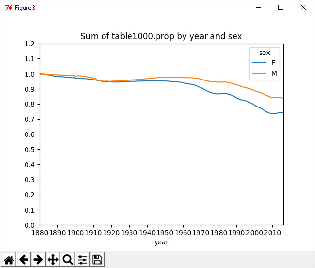
前1000项的比例降低,说明名字的多样性确实出现了增长。
二、计算占总出生人数前50%的不同名字的数量,暂且只考虑2010年男孩的名字。
 1 In [33]: df = boys[boys.year == 2010]
 2
 3 In [34]: df
 4 Out[34]:
 5                name sex  number  year      prop
 6 260877        Jacob   M   22110  2010  0.011544
 7 260878        Ethan   M   17995  2010  0.009395
 8 260879      Michael   M   17336  2010  0.009051
 9 260880       Jayden   M   17163  2010  0.008961
10 260881      William   M   17042  2010  0.008898
11 260882    Alexander   M   16749  2010  0.008745
12 260883         Noah   M   16442  2010  0.008584
13 260884       Daniel   M   15827  2010  0.008263
14 260885        Aiden   M   15531  2010  0.008109
15 260886      Anthony   M   15482  2010  0.008083
16 260887       Joshua   M   15432  2010  0.008057
17 260888        Mason   M   14837  2010  0.007746
18 260889  Christopher   M   14263  2010  0.007447
19 260890       Andrew   M   14234  2010  0.007432
20 260891        David   M   14181  2010  0.007404
21 260892      Matthew   M   14119  2010  0.007372
22 260893        Logan   M   14015  2010  0.007317
23 260894       Elijah   M   13879  2010  0.007246
24 260895        James   M   13870  2010  0.007242
25 260896       Joseph   M   13816  2010  0.007213
26 260897      Gabriel   M   12865  2010  0.006717
27 260898     Benjamin   M   12427  2010  0.006488
28 260899         Ryan   M   11967  2010  0.006248
29 260900       Samuel   M   11954  2010  0.006241
30 260901      Jackson   M   11813  2010  0.006168
31 260902         John   M   11550  2010  0.006030
32 260903       Nathan   M   11368  2010  0.005935
33 260904     Jonathan   M   11116  2010  0.005804
34 260905    Christian   M   11090  2010  0.005790
35 260906         Liam   M   10927  2010  0.005705
36 ...             ...  ..     ...   ...       ...
37 261847      Ronaldo   M     203  2010  0.000106
38 261848         Yair   M     203  2010  0.000106
39 261849       Lathan   M     203  2010  0.000106
40 261850       Gibson   M     202  2010  0.000105
41 261851        Keyon   M     202  2010  0.000105
42 261852       Reagan   M     202  2010  0.000105
43 261853       Daylen   M     201  2010  0.000105
44 261854     Kingsley   M     201  2010  0.000105
45 261855        Talan   M     201  2010  0.000105
46 261856       Yehuda   M     201  2010  0.000105
47 261857       Jordon   M     200  2010  0.000104
48 261858        Slade   M     200  2010  0.000104
49 261859      Sheldon   M     200  2010  0.000104
50 261860      Dashawn   M     200  2010  0.000104
51 261861    Cristofer   M     200  2010  0.000104
52 261862     Clarence   M     199  2010  0.000104
53 261863       Dillan   M     199  2010  0.000104
54 261864        Kadin   M     199  2010  0.000104
55 261865        Masen   M     199  2010  0.000104
56 261866        Rowen   M     199  2010  0.000104
57 261867      Clinton   M     198  2010  0.000103
58 261868     Thaddeus   M     198  2010  0.000103
59 261869       Yousef   M     198  2010  0.000103
60 261870       Truman   M     197  2010  0.000103
61 261871       Joziah   M     196  2010  0.000102
62 261872       Simeon   M     196  2010  0.000102
63 261873       Reuben   M     196  2010  0.000102
64 261874      Keshawn   M     196  2010  0.000102
65 261875      Eliezer   M     196  2010  0.000102
66 261876        Enoch   M     196  2010  0.000102
67
68 [1000 rows x 5 columns]
先计算prop的累积和cumsum,然后再通过searchsorted方法找出0.5应该被插入在哪个位置才能保证不破坏顺序。
 1 In [35]: prop_cumsum = df.sort_values(by='prop', ascending=False).prop.cumsum()
 2
 3 In [36]: prop_cumsum[:10]
 4 Out[36]:
 5 260877    0.011544
 6 260878    0.020939
 7 260879    0.029990
 8 260880    0.038951
 9 260881    0.047849
10 260882    0.056593
11 260883    0.065178
12 260884    0.073441
13 260885    0.081550
14 260886    0.089633
15 Name: prop, dtype: float64
16
17 In [37]: prop_cumsum.searchsorted(0.5)
18 Out[37]: array([116], dtype=int64)
由于数组索引从0开始,因此要给结果+1,即最终结果为117。而1900年的25则要小得多。
1 In [38]: df = boys[boys.year == 1900]
2
3 In [39]: in1900 = df.sort_values(by='prop', ascending=False).prop.cumsum()
4
5 In [40]: in1900.searchsorted(0.5) + 1
6 Out[40]: array([25], dtype=int64)
Error
 1 In [41]: def get_quantile_count(group, q=0.5):
 2    ....:     group = group.sort_values(by='prop', ascending=False)
 3    ....:     return group.prop.cumsum().searchsorted(q) + 1
 4    ....:
 5
 6 In [42]: diversity = top1000.groupby(['year','sex']).apply(get_quantile_count)
 7
 8 In [43]: diversity = diversity.unstack('sex')
 9
10 In [44]: diversity.head()
11 Out[44]:
12 sex      F     M
13 year
14 1880  [38]  [14]
15 1881  [38]  [14]
16 1882  [38]  [15]
17 1883  [39]  [15]
18 1884  [39]  [16]
19
20 In [45]: diversity.plot(title="Number of popular names in top50%")
21 ---------------------------------------------------------------------------
22 TypeError                                 Traceback (most recent call last)
23 <ipython-input-40-d380f36f6920> in <module>()
24 ----> 1 diversity.plot(title="Number of popular names in top50%")
25
26 C:UsersI******AppDataLocalEnthoughtCanopyAppappdatacanopy-2.1.3.3542.win-x86_64libsite-packagespandas-0.20.3-py2.7-win-amd64.eggpandasplotting\_core.pyc in __call__(self, x, y, kind, ax, subplots, sharex, sharey, layout, figsize, use_index, title, grid, legend, style, logx, logy, loglog, xticks, yticks, xlim, ylim, rot, fontsize, colormap, table, yerr, xerr, secondary_y, sort_columns, **kwds)
27    2625                           fontsize=fontsize, colormap=colormap, table=table,
28    2626                           yerr=yerr, xerr=xerr, secondary_y=secondary_y,
29 -> 2627                           sort_columns=sort_columns, **kwds)
30    2628     __call__.__doc__ = plot_frame.__doc__
31    2629
32
33 C:UsersI******AppDataLocalEnthoughtCanopyAppappdatacanopy-2.1.3.3542.win-x86_64libsite-packagespandas-0.20.3-py2.7-win-amd64.eggpandasplotting\_core.pyc in plot_frame(data, x, y, kind, ax, subplots, sharex, sharey, layout, figsize, use_index, title, grid, legend, style, logx, logy, loglog, xticks, yticks, xlim, ylim, rot, fontsize, colormap, table, yerr, xerr, secondary_y, sort_columns, **kwds)
34    1867                  yerr=yerr, xerr=xerr,
35    1868                  secondary_y=secondary_y, sort_columns=sort_columns,
36 -> 1869                  **kwds)
37    1870
38    1871
39
40 C:UsersI******AppDataLocalEnthoughtCanopyAppappdatacanopy-2.1.3.3542.win-x86_64libsite-packagespandas-0.20.3-py2.7-win-amd64.eggpandasplotting\_core.pyc in _plot(data, x, y, subplots, ax, kind, **kwds)
41    1692         plot_obj = klass(data, subplots=subplots, ax=ax, kind=kind, **kwds)
42    1693
43 -> 1694     plot_obj.generate()
44    1695     plot_obj.draw()
45    1696     return plot_obj.result
46
47 C:UsersI******AppDataLocalEnthoughtCanopyAppappdatacanopy-2.1.3.3542.win-x86_64libsite-packagespandas-0.20.3-py2.7-win-amd64.eggpandasplotting\_core.pyc in generate(self)
48     241     def generate(self):
49     242         self._args_adjust()
50 --> 243         self._compute_plot_data()
51     244         self._setup_subplots()
52     245         self._make_plot()
53
54 C:UsersI******AppDataLocalEnthoughtCanopyAppappdatacanopy-2.1.3.3542.win-x86_64libsite-packagespandas-0.20.3-py2.7-win-amd64.eggpandasplotting\_core.pyc in _compute_plot_data(self)
55     350         if is_empty:
56     351             raise TypeError('Empty {0!r}: no numeric data to '
57 --> 352                             'plot'.format(numeric_data.__class__.__name__))
58     353
59     354         self.data = numeric_data
60
61 TypeError: Empty 'DataFrame': no numeric data to plot
Solution01
python3的searchsorted()返回的是ndarray类型而不是int64类型,所以需要先取[0]元素,才能获得想要的数据。
 1 In [46]: def get_quantile_count(group, q=0.5):
 2    ....:     group = group.sort_values(by='prop', ascending=False)
 3    ....:     return group.prop.cumsum().searchsorted(q)[0] + 1
 4    ....:
 5
 6 In [47]: diversity = top1000.groupby(['year', 'sex']).apply(get_quantile_count)
 7
 8 In [48]: diversity = diversity.unstack('sex')
 9
10 In [49]: diversity.head()
11 Out[49]:
12 sex    F   M
13 year
14 1880  38  14
15 1881  38  14
16 1882  38  15
17 1883  39  15
18 1884  39  16
19
20 In [50]: diversity.plot(title="Number of popular names in top50%")
21 Out[50]: <matplotlib.axes._subplots.AxesSubplot at 0xcbce208>
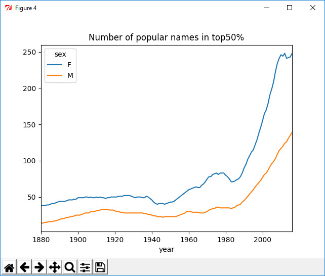
从图中可以看出,女孩名字的多样性总是比男孩的高,而且还在变得越来越高。
最后一个字母
将全部出生数据在年度、性别以及末字母上进行聚合。
 1 In [51]: get_last_letter = lambda x: x[-1]
 2
 3 In [52]: last_letters = names.name.map(get_last_letter)
 4
 5 In [53]: last_letters.name = 'last_letter'
 6
 7 In [54]: table = names.pivot_table('number', index=last_letters, columns=['sex', 'year'], aggfunc=sum)
 8
 9 In [55]: subtable = table.reindex(columns=[1916, 1966, 2016], level='year')
10
11 In [56]: subtable.head()
12 Out[56]:
13 sex                 F                             M
14 year             1916      1966      2016      1916      1966      2016
15 last_letter
16 a            272225.0  616110.0  654193.0    3509.0    4630.0   29454.0
17 b                 NaN     100.0     645.0    1600.0    1732.0   26812.0
18 c                 5.0     145.0    1284.0    1978.0   22036.0   21912.0
19 d             19035.0    3127.0    3418.0  118335.0  209457.0   42748.0
20 e            324987.0  364405.0  324067.0  108122.0  125970.0  125222.0
21
22 In [57]: subtable.sum()
23 Out[57]:
24 sex  year
25 F    1916    1044335.0
26      1966    1691964.0
27      2016    1756647.0
28 M    1916     890100.0
29      1966    1783903.0
30      2016    1880674.0
31 dtype: float64
32
33 In [58]: letter_prop = subtable / subtable.sum().astype(float)
绘图
1 In [59]: import matplotlib.pyplot as plt
2
3 In [60]: fig, axes = plt.subplots(2, 1, figsize=(10, 8))
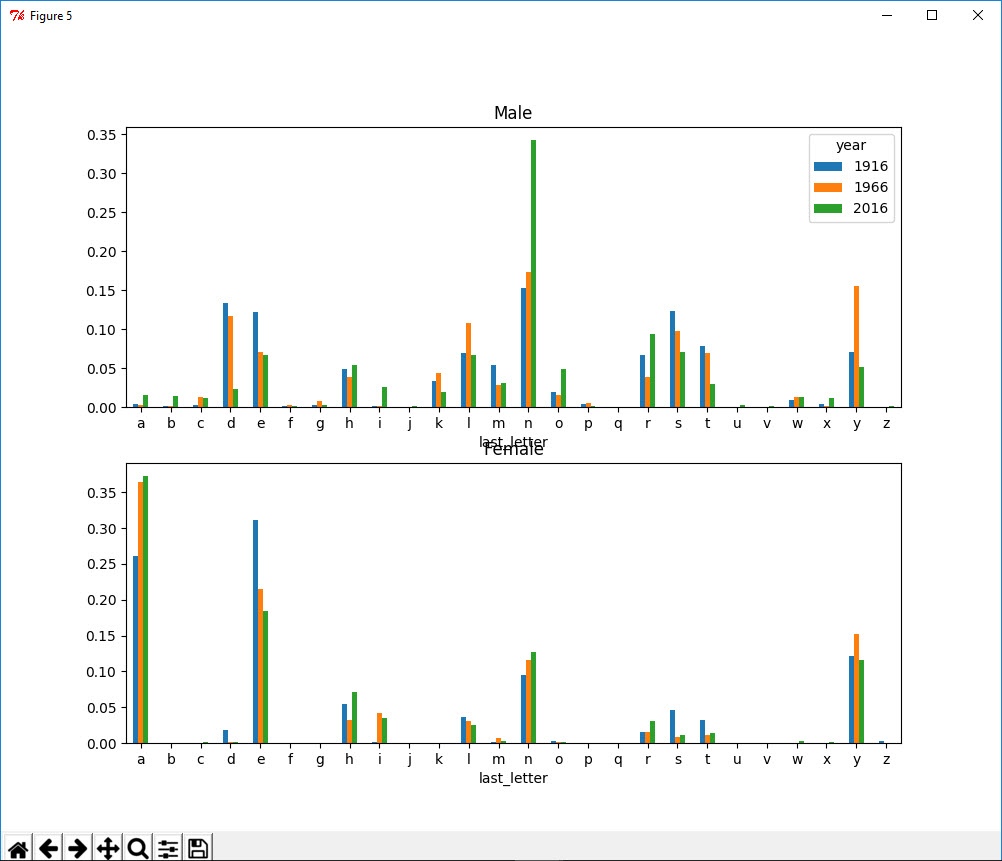
1 In [61]: letter_prop['M'].plot(kind='bar', rot=0, ax=axes[0], title='Male')
2 Out[61]: <matplotlib.axes._subplots.AxesSubplot at 0x3924ad68>
3
4 In [62]: letter_prop['F'].plot(kind='bar', rot=0, ax=axes[1], title='Female', legend=False)
5 Out[62]: <matplotlib.axes._subplots.AxesSubplot at 0x39340438>
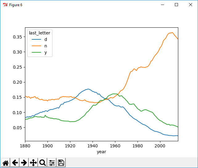
回到之前创建的那个完整的表,按年度和性别对其进行规范化处理,并在男孩名字中选取几个字母,最后进行转置以便将各个列做成一个时间序列。
 1 In [63]: letter_prop = table / table.sum().astype(float)
 2
 3 In [64]: dny_ts = letter_prop.loc[['d', 'n', 'y'], 'M'].T
 4
 5 In [65]: dny_ts.head()
 6 Out[65]:
 7 last_letter         d         n         y
 8 year
 9 1880         0.083057  0.153216  0.075762
10 1881         0.083242  0.153212  0.077455
11 1882         0.085332  0.149561  0.077538
12 1883         0.084051  0.151653  0.079148
13 1884         0.086121  0.149926  0.080407
14
15 In [66]: dny_ts.plot()
16 Out[66]: <matplotlib.axes._subplots.AxesSubplot at 0x3c2737b8>
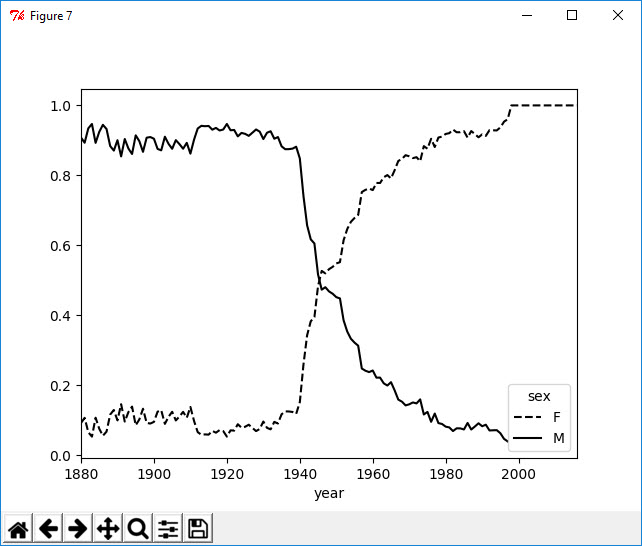
变成女孩名字的男孩名字
 1 In [67]: all_names = top1000.name.unique()
 2
 3 In [68]: mask = np.array(['lesl' in x.lower() for x in all_names])
 4
 5 In [69]: lesley_like = all_names[mask]
 6
 7 In [70]: lesley_like
 8 Out[70]: array(['Leslie', 'Lesley', 'Leslee', 'Lesli', 'Lesly'], dtype=object)
 9
10 In [71]: filtered = top1000[top1000.name.isin(lesley_like)]
11
12 In [72]: filtered.groupby('name').number.sum()
13 Out[72]:
14 name
15 Leslee       993
16 Lesley     35032
17 Lesli        929
18 Leslie    376857
19 Lesly      11432
20 Name: number, dtype: int64
21
22 In [73]: table = filtered.pivot_table('number', index='year', columns='sex', aggfunc='sum')
23
24 In [74]: table = table.div(table.sum(1), axis=0)
25
26 In [75]: table.tail()
27 Out[75]:
28 sex     F   M
29 year
30 2012  1.0 NaN
31 2013  1.0 NaN
32 2014  1.0 NaN
33 2015  1.0 NaN
34 2016  1.0 NaN
35
36 In [76]: table.plot(style={'M': 'k-', 'F': 'k--'})
37 Out[76]: <matplotlib.axes._subplots.AxesSubplot at 0x3b1e2a58>
Reference
01 http://blog.csdn.net/u010456562/article/details/51346594