最终初学者指南，以数据科学用例赢得分类黑客马拉松

作者|VETRIVEL_PS
编译|Flin
来源|analyticsvidhya

总览

本文是我的第一篇Analytics Vidhya的博客文章的第二部分，该文章是进入机器学习黑客马拉松的前10％的终极入门者指南。
如果你遵循本文列出的这些简单步骤，那么赢得黑客马拉松的分类问题就比较简单
始终保持不断的学习，以高度的一致性进行实验，并遵循你的直觉和你随着时间积累的领域知识
从几个月前在Hackathons作为初学者开始，我最近成为了Kaggle专家，并且是 Vidhya 的JanataHack Hackathon系列分析的前5名贡献者之一。
我在这里分享我的知识，并指导初学者使用Binary分类中的分类用例进行顶级黑客竞赛

让我们深入研究二元分类–来自Analytics Vidhya的JanataHack Hackathon系列的保险交叉销售用例，并亲自进行实验

链接到交叉销售黑客马拉松！- https://datahack.analyticsvidhya.com/contest/janatahack-cross-sell-prediction/#ProblemStatement

我们的客户是一家为客户提供健康保险的保险公司。现在他们需要我们的帮助来构建模型，以预测过去一年的保单持有人（客户）是否也会对公司提供的车辆保险感兴趣。

保险单是公司承诺为特定的损失，损害，疾病或死亡提供赔偿保证，以换取指定的保险费的一种安排。保费是客户需要定期向保险公司支付此保证金的金额。

例如，我们每年可以为200000卢比的健康保险支付5000卢比的保险费，这样，如果我们在那一年生病并需要住院治疗，保险公司将承担最高200000卢比的住院费用。现在，如果我们想知道，当公司只收取5000卢比的保险费时，该如何承担如此高的住院费用，那么，概率的概念就出现了。

例如，像我们一样，每年可能有100名客户支付5000卢比的保险费，但只有少数人（比如2-3人）会在当年住院。这样，每个人都会分担其他人的风险。

就像医疗保险一样，有些车辆保险每年需要客户向保险提供商公司支付一定金额的保险费，这样，如果车辆不幸发生意外，保险提供商公司将提供赔偿（称为“投保”）。

建立模型来预测客户是否会对车辆保险感兴趣对公司非常有帮助，因为它随后可以相应地计划其沟通策略，以覆盖这些客户并优化其业务模型和收入。

分享我的数据科学黑客马拉松方法——如何在20,000多个数据爱好者中达到前10％

在第1部分中，我们学习可以重复，优化和改进的10个步骤，这是帮助你快速入门的良好基础。

现在你已经开始练习，让我们尝试保险用例来测试我们的技能。放心，你将在几个星期的练习中很好地应对任何分类黑客马拉松（带有表格数据）。希望你热情，好奇，并通过黑客竞赛继续这一数据科学之旅！

学习，练习和分类黑客马拉松的10个简单步骤

1. 理解问题陈述并导入包和数据集

2. 执行EDA（探索性数据分析）——了解数据集。探索训练和测试数据，并了解每个列/特征表示什么。检查数据集中目标列是否不平衡

3. 从训练数据检查重复的行

4. 填充/插补缺失值-连续-平均值/中值/任何特定值|分类-其他/正向填充/回填

5. 特征工程–特征选择–选择最重要的现有特征| 特征创建或封装–从现有特征创建新特征

6. 将训练数据拆分为特征（独立变量）| 目标（因变量）

7. 数据编码–目标编码，独热编码|数据缩放–MinMaxScaler，StandardScaler，RobustScaler

8. 为二进制分类问题创建基线机器学习模型

9. 结合平均值使用K折交叉验证改进评估指标“ ROC_AUC”并预测目标“Response”

10. 提交结果，检查排行榜并改进“ ROC_AUC”

在GitHub链接上查看PYTHON中完整的工作代码以及可用于学习和练习的输出。只要进行更改，它就会更新！

https://github.com/Vetrivel-PS/AV-JanataHack-Insurance-Cross-Sell/blob/main/Latest-AV-Cross-Sell-Post-Hackathon-Analysis-3-ML-Models-in-GPU.ipynb

1. 了解问题陈述并导入包和数据集

数据集说明

变量	说明
id	客户的唯一ID
Gender	客户性别
Age	客户年龄
Driving_License	0：客户没有驾照 1：客户已经有驾照
Region_Code	客户所在地区的唯一代码
Previously_Insured	1：客户已经有车辆保险 0：客户没有车辆保险
Vehicle_Age	车龄
Vehicle_Damage	1：客户过去曾损坏车辆 0：客户过去未曾损坏车辆。
Annual_Premium	客户需要在当年支付的保费金额
Policy_Sales_Channel	与客户联系的渠道的匿名代码，即不同的代理，通过邮件，通过电话，见面等
Vintage	客户已与公司建立联系的天数
Response	1：客户感兴趣 0：客户不感兴趣

现在，为了预测客户是否会对车辆保险感兴趣，我们获得了有关人口统计信息（性别，年龄，区域代码类型），车辆（车辆年龄，损坏），保单（保险费，采购渠道）等信息。

用于检查所有Hackathon中机器学习模型性能差异的评估指标

在这里，我们将ROC_AUC作为评估指标。

受试者工作特征曲线（ROC）是用于二元分类问题的评价度量。这是一条概率曲线，绘制了各种阈值下的TPR（真阳性率）对FPR（假阳性率），并从本质上将“信号”与“噪声”分开。所述的曲线下面积（AUC）是一个分类类别之间进行区分的能力的量度，并且被用作ROC曲线的总结。

AUC越高，模型在区分正类和负类方面的性能越好。

当AUC=1时，分类器能够正确区分所有的正类点和负类点。然而，如果AUC为0，那么分类器将预测所有的阴性为阳性，所有的阳性为阴性。
当0.5 < AUC < 1时，分类器很有可能将正类别值与负类别值区分开。之所以如此，是因为与假阴性和假阳性相比，分类器能够检测更多数量的真阳性和真阴性。
当AUC = 0.5时，分类器无法区分正类别点和负类别点。这意味着分类器将为所有数据点预测随机类别或常量类别。
交叉销售：训练数据包含3,81,109个示例，测试数据包含1,27,037个示例。数据再次出现严重失衡——根据训练数据，仅推荐12.2％（总计3,81,109名员工中的46,709名）晋升。

让我们从导入所需的Python包开始

# Import Required Python Packages
# Scientific and Data Manipulation Libraries
import numpy as np
import pandas as pd

# Data Viz & Regular Expression Libraries
import matplotlib.pyplot as plt
import seaborn as sns

# Scikit-Learn Pre-Processing Libraries
from sklearn.preprocessing import *

# Garbage Collection Libraries
import gc

# Boosting Algorithm Libraries
from xgboost import XGBClassifier
from catboost import CatBoostClassifier
from lightgbm import LGBMClassifier

# Model Evaluation Metric & Cross Validation Libraries
from sklearn.metrics import roc_auc_score, auc, roc_curve
from sklearn.model_selection import StratifiedKFold, KFold

# Setting SEED to Reproduce Same Results even with "GPU"
seed_value = 1994
import os
os.environ['PYTHONHASHSEED'} = str(seed_value)
import random
random.seed(seed_value)
import numpy as np
np.random.seed(seed_value)
SEED=seed_value

科学和数据处理 ——用于使用Numpy处理数字数据，使用Pandas处理表格数据。
数据可视化库——Matplotlib和Seaborn用于可视化单个或多个变量。
数据预处理，机器学习和度量标准库——用于通过使用评估度量标准（例如ROC_AUC分数）通过编码，缩放和测量日期来预处理数据。
提升算法– XGBoost，CatBoost和LightGBM基于树的分类器模型用于二进制以及多类分类
设置SEED –用于将SEED设置为每次重现相同的结果

2. 执行EDA（探索性数据分析）–了解数据集

# Loading data from train, test and submission csv files
train = pd.read_csv('../input/avcrosssellhackathon/train.csv')
test = pd.read_csv('../input/avcrosssellhackathon/test.csv')
sub = pd.read_csv('../input/avcrosssellhackathon/sample_submission.csv')

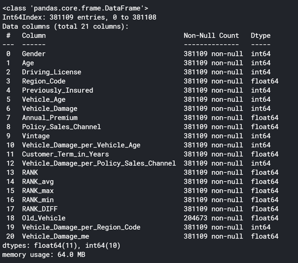
# Python Method 1 : Displays Data Information
def display_data_information(data, data_types, df)
data.info()
print("
")
for VARIABLE in data_types :
data_type = data.select_dtypes(include=[ VARIABLE }).dtypes
if len(data_type) > 0 :
print(str(len(data_type))+" "+VARIABLE+" Features
"+str(data_type)+"
" )

# Display Data Information of "train" :
data_types = ["float32","float64","int32","int64","object","category","datetime64[ns}"}
display_data_information(train, data_types, "train")

# Display Data Information of "test" :
display_data_information(test, data_types, "test")

# Python Method 2 : Displays Data Head (Top Rows) and Tail (Bottom Rows) of the Dataframe (Table) :
def display_head_tail(data, head_rows, tail_rows)
display("Data Head & Tail :")
display(data.head(head_rows).append(data.tail(tail_rows)))

#     return True
# Displays Data Head (Top Rows) and Tail (Bottom Rows) of the Dataframe (Table)
# Pass Dataframe as "train", No. of Rows in Head = 3 and No. of Rows in Tail = 2 :
display_head_tail(train, head_rows=3, tail_rows=2)

# Python Method 3 : Displays Data Description using Statistics :
def display_data_description(data, numeric_data_types, categorical_data_types)
print("Data Description :")
display(data.describe( include = numeric_data_types))
print("")
display(data.describe( include = categorical_data_types))

# Display Data Description of "train" :
display_data_description(train, data_types[0:4}, data_types[4:7})

# Display Data Description of "test" :
display_data_description(test, data_types[0:4}, data_types[4:7})

读取CSV格式的数据文件——pandas的read_csv方法，用于读取csv文件，并转换成类似Data结构的表，称为DataFrame。因此，为训练，测试和提交创建了3个数据帧。

在数据上应用头尾 –用于查看前3行和后2行以获取数据概览。

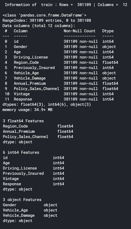
在数据上应用信息–用于显示有关数据帧的列，数据类型和内存使用情况的信息。

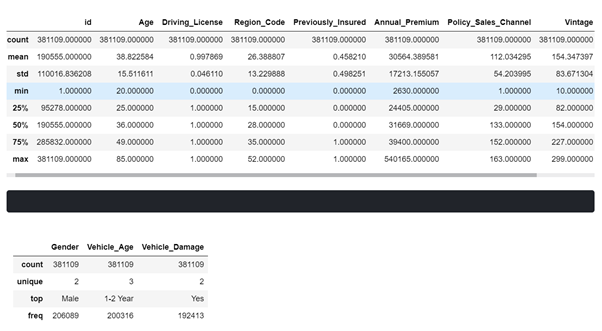
在数据上应用描述–用于在数字列上显示描述统计信息，例如计数，唯一性，均值，最小值，最大值等。

3. 从训练数据检查重复的行

# Removes Data Duplicates while Retaining the First one
def remove_duplicate(data)
data.drop_duplicates(keep="first", inplace=True)
return "Checked Duplicates
# Removes Duplicates from train data
remove_duplicate(train)

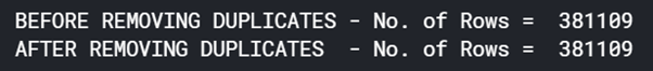
检查训练数据是否重复——通过保留第一行来删除重复的行。在训练数据中找不到重复项。

4. 填充/插补缺失值-连续-平均值/中值/任何特定值|分类-其他/正向填充/回填

数据中没有缺失值。

5. 特征工程

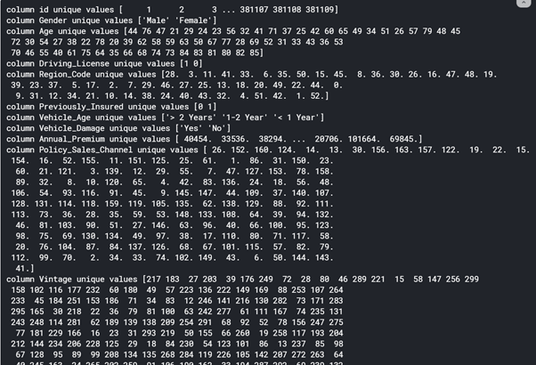
# Check train data for Values of each Column - Short Form
for i in train
print(f'column {i} unique values {train[i}.unique()})

# Binary Classification Problem - Target has ONLY 2 Categories
# Target - Response has 2 Values of Customers 1 & 0
# Combine train and test data into single DataFrame - combine_set
combine_set = pd.concat{[train,test},axis=0}
# converting object to int type :
combine_set['Vehicle_Age'}=combine_set['Vehicle_Age'}.replacee({'< 1 Year':0,'1-2 Year':1,'> 2 Years':2})
combine_set['Gender'}=combine_set['Gender'}.replacee({'Male':1,'Female':0})
combine_set['Vehicle_Damage'}=combine_set['Vehicle_Damage'}.replacee({'Yes':1,'No':0})
sns.heatmap(combine_set.corr())

# HOLD - CV - 0.8589 - BEST EVER
combine_set['Vehicle_Damage_per_Vehicle_Age'} = combine_set.groupby(['Region_Code,Age'})['Vehicle_Damage'}.transform('sum'
# Score - 0.858657 (This Feature + Removed Scale_Pos_weight in LGBM) | Rank - 20
combine_set['Customer_Term_in_Years'} = combine_set['Vintage'} / 365
# combine_set['Customer_Term'} = (combine_set['Vintage'} / 365).astype('str')
# Score - 0.85855 | Rank - 20
combine_set['Vehicle_Damage_per_Policy_Sales_Channel'} = combine_set.groupby(['Region_Code,Policy_Sales_Channel'})['Vehicle_Damage'}.transform('sum')
# Score - 0.858527 | Rank - 22
combine_set['Vehicle_Damage_per_Vehicle_Age'} = combine_set.groupby(['Region_Code,Vehicle_Age'})['Vehicle_Damage'}.transform('sum')
# Score - 0.858510 | Rank - 23
combine_set["RANK"} = combine_set.groupby("id")['id'}.rank(method="first", ascending=True)
combine_set["RANK_avg"} = combine_set.groupby("id")['id'}.rank(method="average", ascending=True)
combine_set["RANK_max"} = combine_set.groupby("id")['id'}.rank(method="max", ascending=True)
combine_set["RANK_min"} = combine_set.groupby("id")['id'}.rank(method="min", ascending=True)
combine_set["RANK_DIFF"} = combine_set['RANK_max'} - combine_set['RANK_min'}
# Score - 0.85838 | Rank - 15
combine_set['Vehicle_Damage_per_Vehicle_Age'} = combine_set.groupby([Region_Code})['Vehicle_Damage'}.transform('sum')

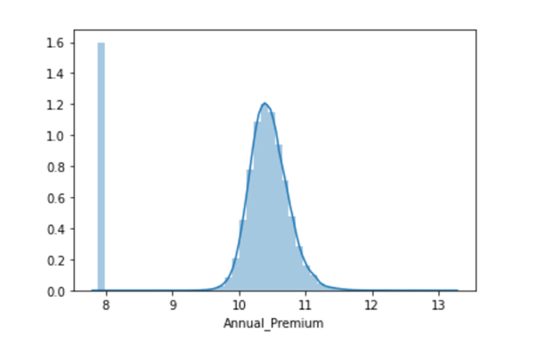
# Data is left Skewed as we can see from below distplot
sns.distplot(combine_set['Annual_Premium'})

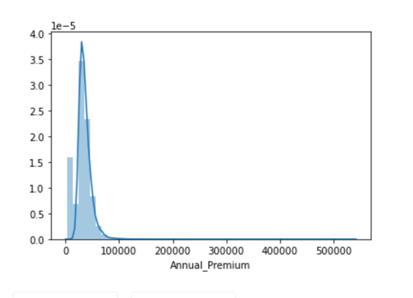
combine_set['Annual_Premium'} = np.log(combine_set['Annual_Premium'})
sns.distplot(combine_set['Annual_Premium'})

# Getting back Train and Test after Preprocessing :
train=combine_set[combine_set['Response'}.isnull()==False}
test=combine_set[combine_set['Response'}.isnull()==True}.drop(['Response'},axis=1)
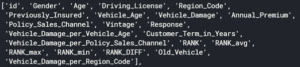
train.columns

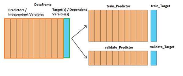
6. 将训练数据拆分为特征（独立变量）| 目标（因变量）

# Split the Train data into predictors and target :
predictor_train = train.drop(['Response','id'],axis=1)
target_train    = train['Response']
predictor_train.head()

# Get the Test data by dropping 'id' :
predictor_test = test.drop(['id'],axis=1)

7. 数据编码–目标编码

def add_noise(series, noise_level):
return series * (1 + noise_level * np.random.randn(len(series)))
def target_encode(trn_series=None,
tst_series=None,
target=None,
min_samples_leaf=1,
smoothing=1,
noise_level=0):
"""
Smoothing is computed like in the following paper by Daniele Micci-Barreca
https://kaggle2.blob.core.windows.net/forum-message-attachments/225952/7441/high%20cardinality%20categoricals.pdf

trn_series : training categorical feature as a pd.Series
tst_series : test categorical feature as a pd.Series
target : target data as a pd.Series
min_samples_leaf (int) : minimum samples to take category average into account
smoothing (int) : smoothing effect to balance categorical average vs prior
"""
assert len(trn_series) == len(target)
assert trn_series.name == tst_series.name
temp = pd.concat([trn_series, target], axis=1)
# Compute target mean
averages = temp.groupby(by=trn_series.name)[target.name].agg(["mean", "count"])
# Compute smoothing
smoothing = 1 / (1 + np.exp(-(averages["count"] - min_samples_leaf) / smoothing))
# Apply average function to all target data
prior = target.mean()
# The bigger the count the less full_avg is taken into account
averages[target.name] = prior * (1 - smoothing) + averages["mean"] * smoothing
averages.drop(["mean", "count"], axis=1, inplace=True)
# Apply averages to trn and tst series
ft_trn_series = pd.merge(
trn_series.to_frame(trn_series.name),
averages.reset_index().rename(columns={'index': target.name, target.name: 'average'}),
on=trn_series.name,
how='left')['average'].rename(trn_series.name + '_mean').fillna(prior)
# pd.merge does not keep the index so restore it
ft_trn_series.index = trn_series.index
ft_tst_series = pd.merge(
tst_series.to_frame(tst_series.name),
averages.reset_index().rename(columns={'index': target.name, target.name: 'average'}),
on=tst_series.name,
how='left')['average'].rename(trn_series.name + '_mean').fillna(prior)
# pd.merge does not keep the index so restore it
ft_tst_series.index = tst_series.index
return add_noise(ft_trn_series, noise_level), add_noise(ft_tst_series, noise_level)
# Score - 0.85857 | Rank -
tr_g, te_g = target_encode(predictor_train["Vehicle_Damage"],
predictor_test["Vehicle_Damage"],
target= predictor_train["Response"],
min_samples_leaf=200,
smoothing=20,
noise_level=0.02)
predictor_train['Vehicle_Damage_me']=tr_g
predictor_test['Vehicle_Damage_me']=te_g

8. 为二进制分类问题创建基线机器学习模型

# Baseline Model Without Hyperparameters :
Classifiers = {'0.XGBoost' : XGBClassifier(),
'1.CatBoost' : CatBoostClassifier(),
'2.LightGBM' : LGBMClassifier()
}
# Fine Tuned Model With-Hyperparameters :
Classifiers = {'0.XGBoost' : XGBClassifier(eval_metric='auc',

# GPU PARAMETERS #
tree_method='gpu_hist',
gpu_id=0,

# GPU PARAMETERS #
random_state=294,
learning_rate=0.15,
max_depth=4,
n_estimators=494,
objective='binary:logistic'),
'1.CatBoost' : CatBoostClassifier(eval_metric='AUC',

# GPU PARAMETERS #
task_type='GPU',
devices="0",

# GPU PARAMETERS #
learning_rate=0.15,
n_estimators=494,
max_depth=7,
#                             scale_pos_weight=2),

'2.LightGBM' : LGBMClassifier(metric = 'auc',

# GPU PARAMETERS #
device = "gpu",
gpu_device_id =0,
max_bin = 63,
gpu_platform_id=1,

# GPU PARAMETERS #
n_estimators=50000,
bagging_fraction=0.95,
subsample_freq = 2,
objective ="binary",
min_samples_leaf= 2,
importance_type = "gain",
verbosity = -1,
random_state=294,
num_leaves = 300,
boosting_type = 'gbdt',
learning_rate=0.15,
max_depth=4,

# scale_pos_weight=2, # Score - 0.85865 | Rank - 18
n_jobs=-1)
}

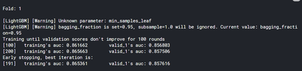
9. 结合平均值使用K折交叉验证改进评估指标“ ROC_AUC”并预测目标“Response”

# LightGBM Model
kf=KFold(n_splits=10,shuffle=True)
preds_1   = list()
y_pred_1  = []
rocauc_score = []
for i,(train_idx,val_idx) in enumerate(kf.split(predictor_train)):
X_train, y_train = predictor_train.iloc[train_idx,:], target_train.iloc[train_idx]
X_val, y_val = predictor_train.iloc[val_idx, :], target_train.iloc[val_idx]
print('
Fold: {}
'.format(i+1))
lg= LGBMClassifier(      metric = 'auc',

# GPU PARAMETERS #
device = "gpu",
gpu_device_id =0,
max_bin = 63,
gpu_platform_id=1,

# GPU PARAMETERS #
n_estimators=50000,
bagging_fraction=0.95,
subsample_freq = 2,
objective ="binary",
min_samples_leaf= 2,
importance_type = "gain",
verbosity = -1,
random_state=294,
num_leaves = 300,
boosting_type = 'gbdt',
learning_rate=0.15,
max_depth=4,
# scale_pos_weight=2, # Score - 0.85865 | Rank - 18
n_jobs=-1
)
lg.fit(X_train, y_train
,eval_set=[(X_train, y_train),(X_val, y_val)]
,early_stopping_rounds=100
,verbose=100
)
roc_auc = roc_auc_score(y_val,lg.predict_proba(X_val)[:, 1])
rocauc_score.append(roc_auc)
preds_1.append(lg.predict_proba(predictor_test [predictor_test.columns])[:, 1])
y_pred_final_1          = np.mean(preds_1,axis=0)
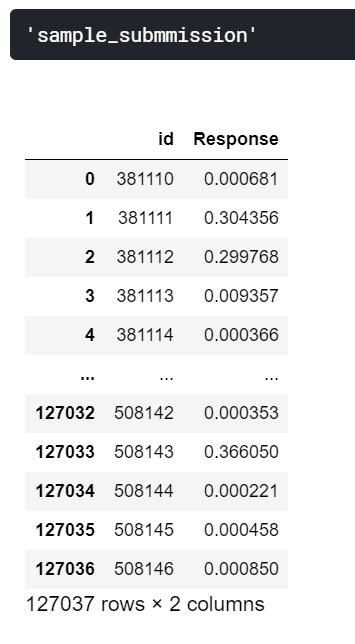
sub['Response']=y_pred_final_1
Blend_model_1 = sub.copy()

print('ROC_AUC - CV Score: {}'.format((sum(rocauc_score)/10)),'
')
print("Score : ",rocauc_score)

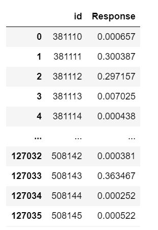
# Download and Show Submission File :
display("sample_submmission",sub)
sub_file_name_1 = "S1. LGBM_GPU_TargetEnc_Vehicle_Damage_me_1994SEED_NoScaler.csv"
sub.to_csv(sub_file_name_1,index=False)
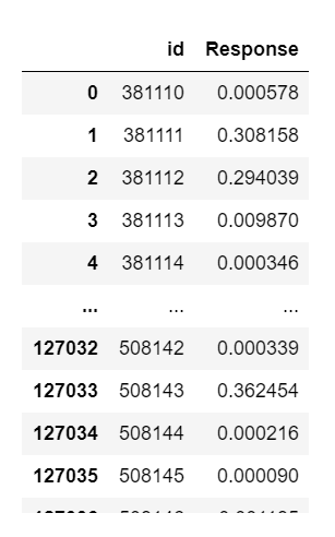
sub.head(5)

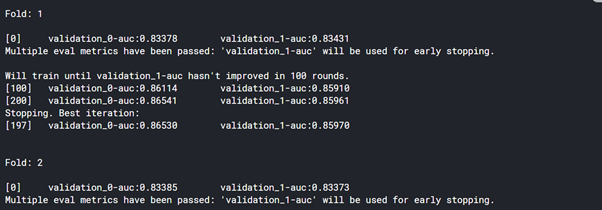
# Catboost Model
kf=KFold(n_splits=10,shuffle=True)
preds_2   = list()
y_pred_2  = []
rocauc_score = []
for i,(train_idx,val_idx) in enumerate(kf.split(predictor_train)):
X_train, y_train = predictor_train.iloc[train_idx,:], target_train.iloc[train_idx]
X_val, y_val = predictor_train.iloc[val_idx, :], target_train.iloc[val_idx]
print('
Fold: {}
'.format(i+1))
cb = CatBoostClassifier( eval_metric='AUC',

# GPU PARAMETERS #
task_type='GPU',
devices="0",

# GPU PARAMETERS #
learning_rate=0.15,
n_estimators=494,
max_depth=7,
#                             scale_pos_weight=2
)
cb.fit(X_train, y_train
,eval_set=[(X_val, y_val)]
,early_stopping_rounds=100
,verbose=100
)
roc_auc = roc_auc_score(y_val,cb.predict_proba(X_val)[:, 1])
rocauc_score.append(roc_auc)
preds_2.append(cb.predict_proba(predictor_test [predictor_test.columns])[:, 1])
y_pred_final_2          = np.mean(preds_2,axis=0)
sub['Response']=y_pred_final_2

print('ROC_AUC - CV Score: {}'.format((sum(rocauc_score)/10)),'
')
print("Score : ",rocauc_score)

# Download and Show Submission File :
display("sample_submmission",sub)
sub_file_name_2 = "S2. CB_GPU_TargetEnc_Vehicle_Damage_me_1994SEED_LGBM_NoScaler_MyStyle.csv"
sub.to_csv(sub_file_name_2,index=False)
Blend_model_2 = sub.copy()
sub.head(5)

# XGBOOST Model
kf=KFold(n_splits=10,shuffle=True)
preds_3   = list()
y_pred_3  = []
rocauc_score = []
for i,(train_idx,val_idx) in enumerate(kf.split(predictor_train)):
X_train, y_train = predictor_train.iloc[train_idx,:], target_train.iloc[train_idx]
X_val, y_val = predictor_train.iloc[val_idx, :], target_train.iloc[val_idx]
print('
Fold: {}
'.format(i+1))
xg=XGBClassifier( eval_metric='auc',

# GPU PARAMETERS #
tree_method='gpu_hist',
gpu_id=0,

# GPU PARAMETERS #
random_state=294,
learning_rate=0.15,
max_depth=4,
n_estimators=494,
objective='binary:logistic'
)
xg.fit(X_train, y_train
,eval_set=[(X_train, y_train),(X_val, y_val)]
,early_stopping_rounds=100
,verbose=100
)
roc_auc = roc_auc_score(y_val,xg.predict_proba(X_val)[:, 1])
rocauc_score.append(roc_auc)
preds_3.append(xg.predict_proba(predictor_test [predictor_test.columns])[:, 1])
y_pred_final_3         = np.mean(preds_3,axis=0)
sub['Response']=y_pred_final_3

print('ROC_AUC - CV Score: {}'.format((sum(rocauc_score)/10)),'
')
print("Score : ",rocauc_score)

# Download and Show Submission File :
display("sample_submmission",sub)
sub_file_name_3 = "S3. XGB_GPU_TargetEnc_Vehicle_Damage_me_1994SEED_LGBM_NoScaler.csv"
sub.to_csv(sub_file_name_3,index=False)
Blend_model_3 = sub.copy()
sub.head(5)

10. 提交结果，检查排行榜并改进“ ROC_AUC”

one = Blend_model_2['id'].copy()
Blend_model_1.drop("id", axis=1, inplace=True)
Blend_model_2.drop("id", axis=1, inplace=True)
Blend_model_3.drop("id", axis=1, inplace=True)
Blend = (Blend_model_1 + Blend_model_2 + Blend_model_3)/3
id_df = pd.DataFrame(one, columns=['id'])
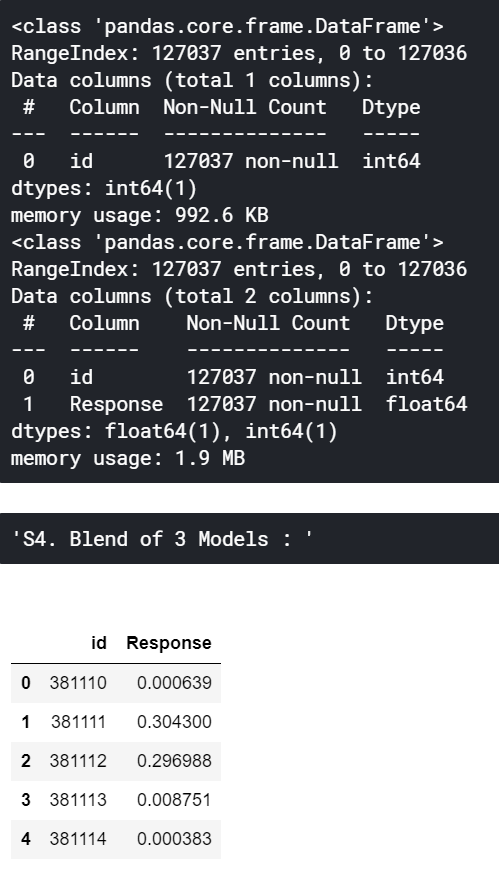
id_df.info()
Blend = pd.concat([ id_df,Blend], axis=1)
Blend.info()
Blend.to_csv('S4. Blend of 3 Models - LGBM_CB_XGB.csv',index=False)
display("S4. Blend of 3 Models : ",Blend.head())

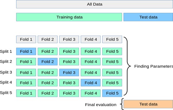
k折交叉验证

交叉验证是一种重采样过程，用于在有限的数据样本上评估机器学习模型。该过程有一个名为k的参数，它表示给定数据样本要分成的组数。因此，这个过程通常被称为k折交叉验证。

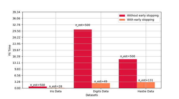
提前停止

在机器学习中，提前停止是一种正则化形式，用于在使用迭代方法（例如梯度下降）训练学习者时避免过拟合。
提前停止规则提供了关于学习者开始过拟合之前可以运行多少次迭代的指导。
文档- https://scikit-learn.org/stable/auto_examples/ensemble/plot_gradient_boosting_early_stopping.html

如何使GPU上的3种机器学习模型运行得更快

LIGHTGBM中的GPU参数
- https://lightgbm.readthedocs.io/en/latest/GPU-Performance.html

要使用LightGBM GPU模型：必须启用“ Internet” –运行以下所有代码：


# 保持Internet处于“打开”状态，该状态位于Kaggle内核的右侧->“设置”面板中

# Cell 1：

!rm -r /opt/conda/lib/python3.6/site-packages/lightgbm

!git clone –recursive https://github.com/Microsoft/LightGBM

# Cell 2：

!apt-get install -y -qq libboost-all-dev

# Cell 3：

%% bash

cd LightGBM

rm -r build

mkdir build

cd build

cmake -DUSE_GPU=1 -DOpenCL_LIBRARY=/usr/local/cuda/lib64/libOpenCL.so -DOpenCL_INCLUDE_DIR=/usr/local/cuda/include/ ..

make -j$(nproc)

# Cell 4：

!cd LightGBM/python-package/;python3 setup.py install –precompile

# Cell 5：

!mkdir -p /etc/OpenCL/vendors && echo “libnvidia-opencl.so.1” > /etc/OpenCL/vendors/nvidia.icd

!rm -r LightGBM

device = “gpu”
gpu_device_id =0
max_bin = 63
gpu_platform_id=1

如何在GPU上实现良好的速度

你想运行一些经过我们验证且具有良好加速性能的数据集（包括Higgs, epsilon, Bosch等），以确保设置正确。如果你有多个GPU，请确保将gpu_platform_id和gpu_device_id设置为使用所需的GPU。还要确保你的系统处于空闲状态（尤其是在使用共享计算机时），以进行准确性性能测量。
GPU在大规模和密集数据集上表现最佳。如果数据集太小，则在GPU上进行计算效率不高，因为数据传输开销可能很大。如果你具有分类功能，请使用categorical_column选项并将其直接输入到LightGBM中。不要将它们转换为独热变量。
为了更好地利用GPU，建议使用较少数量的bin。建议设置max_bin = 63，因为它通常不会明显影响大型数据集上的训练精度，但是GPU训练比使用默认bin大小255明显快得多。对于某些数据集，即使使用15个bin也就足够了（max_bin = 15 ）; 使用15个bin将最大化GPU性能。确保检查运行日志并验证是否使用了所需数量的bin。
尽可能尝试使用单精度训练（gpu_use_dp = false），因为大多数GPU（尤其是NVIDIA消费类GPU）的双精度性能都很差。

2. CATBOOST中的GPU参数

task_type=’GPU’
devices=”0″

参数	描述
CatBoost (fit)	task_type:用于训练的处理单元类型。可能的值：(1)中央处理器(2)GPU
CatBoostClassifier(fit) CatBoostRegressor(fit)	设备:用于训练的GPU设备的ID（索引从零开始）。格式: (1)一台设备的（例如3） (2)<多个设备的：：..：（例如，devices ='0：1：3'） (3)<设备ID1>-<设备IDN>用于一系列设备（例如，devices ='0-3'）

3. XGBOOST中的GPU参数

tree_method ='gpu_hist'
gpu_id = 0

用法

将tree_method参数指定为以下算法之一。

演算法

tree_method	描述
gpu_hist	等效于XGBoost快速直方图算法。它快得多，并使用更少的内存。注意：在比Pascal架构更早的GPU上运行可能会非常缓慢。

支持的参数

参数	gpu_hist
subsample	✔
sampling_method	✔
colsample_bytree	✔
colsample_bylevel	✔
max_bin	✔
gamma	✔
gpu_id	✔
predictor	✔
grow_policy	✔
monotone_constraints	✔
interaction_constraints	✔
single_precision_histogram	✔

黑客马拉松交叉销售总结

在这个AV交叉销售黑客竞赛中起作用的“10件事”：

2个最佳功能：Vehicle_Damage的目标编码和按Region_Code分组的Vehicle_Damage总和——基于特征重要性-在CV（10折交叉验证）和LB（公共排行榜）方面有了很大提升。
基于域的特征：旧车辆的频率编码——有所提高。LB得分：0.85838 |LB排名：15
Hackathon Solutions的排名功能：带来了巨大的推动力。LB得分：0.858510 |LB排名：23
删除“id”栏：带来了巨大的推动力。
基于域的特性：每辆车辆的车辆损坏、年龄和地区代码——有一点提升。LB得分：0.858527 |LB排名：22
消除年度保险费的偏离值：带来了巨大的推动力。 LB得分： 0.85855 |LB排名： 20
基于领域的特征：每个地区的车辆损坏，代码和政策，销售渠道，基于特征重要性，有一点提升。LB得分：0.85856 |LB排名：20
用超参数和10-Fold CV对所有3个模型进行了调整，得出了一个稳健的策略和最好的结果，早期停止的轮数=50或100。Scale_pos_weight在这里没有太大作用。
基于域的特性：客户期限以年为单位，因为其他特性也以年为单位，保险响应将基于年数。LB得分：0.858657 |LB排名：18
综合/混合所有3个最好的单独模型：LightGBM、CatBoost和XGBoost，得到了最好的分数。

5件“不管用”的事

未处理的特征：[ 按年龄分组的车辆损坏总和，按以前投保的车辆损坏总和，按地区代码分组的车辆损坏计数，按地区代码分组的车辆最大损坏，按地区代码分组的最小车辆损坏，按老旧车辆的频率编码，车辆年龄的频率编码，每月EMI=年度保险费/12，按保险单分组的车辆损坏总额，按车辆年龄分组的车辆损坏总额，按驾驶执照分组的车辆损坏总额 ]
删除与响应不相关的驾驶执照列
所有特征的独热编码/虚拟编码
与未标度数据相比，所有3种标度方法都不起作用——StandardScaler给出了其中最好的LB评分。StandardScaler –0.8581 | MinMaxScaler–0.8580 | RobustScaler–0.8444
删除基于训练和测试的Region_Code上的重复代码根本不起作用

第2部分结束！（系列待续）

如果你觉得这篇文章有帮助，请与数据科学初学者分享，帮助他们开始黑客竞赛，因为它解释了许多步骤，如基于领域知识的特征工程、交叉验证、提前停止、在GPU中运行3个机器学习模型，对多个模型进行平均组合，最后总结出“哪些技术有效，哪些无效–最后一步将帮助我们节省大量时间和精力。这将提高未来我们对黑客竞赛的关注度。

非常感谢你的阅读！

原文链接：https://www.analyticsvidhya.com/blog/2020/10/ultimate-beginners-guide-to-win-classification-hackathons-with-a-data-science-use-case/

欢迎关注磐创AI博客站：
http://panchuang.net/

sklearn机器学习中文官方文档：
http://sklearn123.com/

欢迎关注磐创博客资源汇总站：
http://docs.panchuang.net/