1.本文的亮度一: 首次提出了Focal loss
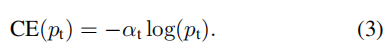
1.解决正负样本分布不均匀,常见的思想是引入一个权重因子α ,α ∈[0,1],当类标签是1(前景),权重因子是α ,当类标签是-1(背景)时,权重因子是1-α 。同样为了表示方便,用αt表示权重因子,那么此时的损失函数被改写为:一般使用at等于0.25,即背景的损失函数是前景的3倍
代码讲解:
alpha_factor = torch.where(torch.eq(targets, 1.), alpha_factor, 1. - alpha_factor) #概率值大于0.5的地方使用 a1, 概率值小于0.4的最大值位置使用1-a1
bce = -(targets * torch.log(classification) + (1.0 - targets) * torch.log(1.0 - classification)) #使用交叉熵损失函数
2.为了解决难易样本的问题,由于在训练过程中无法区分简单样本,容易导致简单样本泛滥的情况,困难样本导致无法学习到,当pt的概率越大时,即(1-pt)的值越小,整体的损失函数也越小,当pt概率越小时,整体的损失函数越大,即复杂的样本更容易分配更多的参数量
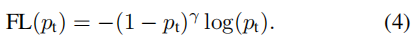
总结: 将上述两个公式进行合并: 就可以得到focal loss 损失函数

上述代码:
focal_weight = torch.where(torch.eq(targets, 1.), 1. - classification, classification) #对于是物体 的使用 1 - pt,对于背景的使用pt
focal_weight = alpha_factor * torch.pow(focal_weight, gamma) #alpha_factor * (1 - p)^y
综上所述: 最终的损失函数是,即
(正样本:)-alpha_factor * (1 - p) * log(p) (阈值大于0.5)
(负样本)-(1 - alpha_factor) * (p) * log(1 - p) (阈值小于0.4, 且离标签IOU最大的位置)
上述cls_loss的完整代码
     IoU = calc_iou(anchors[0, :, :], bbox_annotation[:, :4]) # num_anchors x num_annotations # 计算目标的iou

            IoU_max, IoU_argmax = torch.max(IoU, dim=1) # num_anchors x 1  #计算每个点与5个实际框中的最大IOU的索引值

            #import pdb
            #pdb.set_trace()

            # compute the loss for classification
            targets = torch.ones(classification.shape) * -1

            if torch.cuda.is_available():
                targets = targets.cuda()

            targets[torch.lt(IoU_max, 0.4), :] = 0  # 把IOU_MAX 小于0.4的置为0

            positive_indices = torch.ge(IoU_max, 0.5) #找出IOU大于0.5的索引值

            num_positive_anchors = positive_indices.sum()

            assigned_annotations = bbox_annotation[IoU_argmax, :] # 从中找出对应的数据

            targets[positive_indices, :] = 0 # 把其中其他类比的概率值置为0
            targets[positive_indices, assigned_annotations[positive_indices, 4].long()] = 1 # 把里面对应位置的物体标记为1

            if torch.cuda.is_available():
                alpha_factor = torch.ones(targets.shape).cuda() * alpha
            else:
                alpha_factor = torch.ones(targets.shape) * alpha

            alpha_factor = torch.where(torch.eq(targets, 1.), alpha_factor, 1. - alpha_factor) #其中标签为1的使用alpha_factor, 标签等于0的使用1 - alpha_factor
            focal_weight = torch.where(torch.eq(targets, 1.), 1. - classification, classification) #
            focal_weight = alpha_factor * torch.pow(focal_weight, gamma) #alpha_factor * (1 - p)^y

            bce = -(targets * torch.log(classification) + (1.0 - targets) * torch.log(1.0 - classification)) # 交叉熵损失函数

            # cls_loss = focal_weight * torch.pow(bce, gamma)
            cls_loss = focal_weight * bce #

            if torch.cuda.is_available():
                cls_loss = torch.where(torch.ne(targets, -1.0), cls_loss, torch.zeros(cls_loss.shape).cuda()) # 将cls_loss 等于-1.0的变为0
            else:
                cls_loss = torch.where(torch.ne(targets, -1.0), cls_loss, torch.zeros(cls_loss.shape))

            classification_losses.append(cls_loss.sum()/torch.clamp(num_positive_anchors.float(), min=1.0)) # 计算平均数
这里的回归误差使用的是IOU大于0.5正样本的相对偏移量,这里比较的是anchor与真实样本的偏移量
上述reg_loss的完整代码
    if positive_indices.sum() > 0:
                assigned_annotations = assigned_annotations[positive_indices, :] #

                anchor_widths_pi = anchor_widths[positive_indices]  # 找到其中的
                anchor_heights_pi = anchor_heights[positive_indices]
                anchor_ctr_x_pi = anchor_ctr_x[positive_indices]
                anchor_ctr_y_pi = anchor_ctr_y[positive_indices]

                gt_widths  = assigned_annotations[:, 2] - assigned_annotations[:, 0]
                gt_heights = assigned_annotations[:, 3] - assigned_annotations[:, 1]
                gt_ctr_x   = assigned_annotations[:, 0] + 0.5 * gt_widths
                gt_ctr_y   = assigned_annotations[:, 1] + 0.5 * gt_heights

                # clip widths to 1
                gt_widths  = torch.clamp(gt_widths, min=1) #真实框的长
                gt_heights = torch.clamp(gt_heights, min=1) #真实框的宽

                targets_dx = (gt_ctr_x - anchor_ctr_x_pi) / anchor_widths_pi # 中心点的偏移量dx
                targets_dy = (gt_ctr_y - anchor_ctr_y_pi) / anchor_heights_pi # 中心点的偏移量dy
                targets_dw = torch.log(gt_widths / anchor_widths_pi) # w的log偏移量, 为了降低大框所产生的影响
                targets_dh = torch.log(gt_heights / anchor_heights_pi) #h的log偏移量, 为了降低大框的影响

                targets = torch.stack((targets_dx, targets_dy, targets_dw, targets_dh))
                targets = targets.t()

                if torch.cuda.is_available():
                    targets = targets/torch.Tensor([[0.1, 0.1, 0.2, 0.2]]).cuda()
                else:
                    targets = targets/torch.Tensor([[0.1, 0.1, 0.2, 0.2]])

                negative_indices = 1 + (~positive_indices) # 负样本的标签为2, 正样本的标签为0

                regression_diff = torch.abs(targets - regression[positive_indices, :]) # 回归的误差

                regression_loss = torch.where(
                    torch.le(regression_diff, 1.0 / 9.0),
                    0.5 * 9.0 * torch.pow(regression_diff, 2),
                    regression_diff - 0.5 / 9.0
                )
                regression_losses.append(regression_loss.mean())
            else:
                if torch.cuda.is_available():
                    regression_losses.append(torch.tensor(0).float().cuda())
                else:
                    regression_losses.append(torch.tensor(0).float())
网络结构:使用的FPN特征金字塔结构
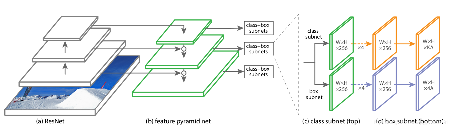
netron网络结构 1 2 3主要用于class+box的预测, 4的分支主要用于前景和背景的概率值预测

github地址: https://github.com/yhenon/pytorch-retinanet