R语言-美国枪杀案分析

案例:该数据集的是一个关于美国2017年犯罪的一个数据集,接下来我们对该数据集进行分析

字段:

####    S# ：数据编号
####    Location：案件发生城市，州
####    Date：时间
####    Summary：案件总结
####    Fatalities：死亡人数
####    Injured：受伤人数
####    Total victims：受害者总人数
####    Mental Health Issues：精神状况
####    Race：种族
####    Gender：性别
####    Latitude：纬度
####    Longitude：经度

1.导入包

library(tidyverse)
library(stringr)
library(data.table)
library(maps)
library(lubridate)
library(leaflet)

2.导入并查看数据集

shooting <- read.csv('Mass Shootings Dataset Ver 2.csv',stringsAsFactors = F,header = T)
summary(shooting)
glimpse(shooting)

　　结论:一共是320行数据,13个变量数据量不大,但是要对数据进行重构

3.数据重构

# 将Date字段进行转化,同时创建新的变量year
shooting <- shooting %>% select(1:13) %>% mutate(Date=mdy(shooting$Date),year=year(Date))
summary(shooting$year)

# 对性别进行提取
shooting$Gender<-if_else(shooting$Gender=="M","Male",shooting$Gender)
# 对种族字段进行提取
shooting$Race<-if_else(str_detect(shooting$Race,"Black American or African American"),"Black",shooting$Race)
shooting$Race<-if_else(str_detect(shooting$Race,"White American or European American"),"White",shooting$Race)
shooting$Race<-if_else(str_detect(shooting$Race,"Asian American"),"Asian",shooting$Race)
shooting$Race<-if_else(str_detect(shooting$Race,"Some other race"),"Other",shooting$Race)
shooting$Race<-if_else(str_detect(shooting$Race,"Native American or Alaska Native"),"Native American",shooting$Race)
# 对时间数据进行切分
shooting$yearcut<-cut(shooting$year,breaks = 10)
# 对是否有心理疾病进行处理
shooting$Mental.Health.Issues<-if_else(str_detect(shooting$Mental.Health.Issues,"Un"),"Unknown",shooting$Mental.Health.Issues)
shooting$Race<-str_to_upper(shooting$Race)
shooting$Mental.Health.Issues<-str_to_upper(shooting$Mental.Health.Issues)
# 把location分解成city和state两个变量
shooting$city <- sapply(shooting$Location,function(x){
  return(unlist(str_split(x,','))[1] %>% str_trim())
})

shooting$state <- sapply(shooting$Location,function(x){
  return(unlist(str_split(x,','))[2] %>% str_trim())
})

4.EDA分析

　　4.1每年的枪击的死亡人数的变化

# 每年受到枪击的死亡人数
shooting %>% 
   group_by(year) %>%
   summarise(total=sum(Total.victims)) %>%
   ggplot(aes(x=year,y=total)) +
   geom_bar(stat = 'identity',fill='blue') +
   geom_text(aes(label=total),vjust=-0.2) +
   xlim(1969,2020) +
   geom_line(color='red') +
   ylab('Total victims every year') +
   ggtitle('People died because of gun shoot every year')

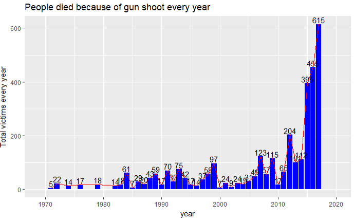
　　结论:在2015年之后,美国的枪击案频发,2017年的因为枪击案的死亡人数上升特别明显

　　4.2 发生枪击案的地点

# 受伤人数的地理位置分布
shooting %>%
  select(Total.victims,Fatalities,Longitude,Latitude,Summary) %>%
  na.omit() %>%
  leaflet() %>%
  addProviderTiles(providers$OpenStreetMap) %>%
  fitBounds(-124,30,-66,43) %>%
  addCircles(color='#8A0707',lng = ~Longitude,lat = ~Latitude,weight = 1,
             radius = ~sqrt(Total.victims) * 20000,popup = ~Summary)

# 死亡人数的地理位置分布
shooting %>%
  select(Total.victims,Fatalities,Longitude,Latitude,Summary) %>%
  na.omit() %>%
  leaflet() %>%
  addProviderTiles(providers$OpenStreetMap) %>%
  fitBounds(-124,30,-66,43) %>%
  addCircles(color='blue',lng = ~Longitude,lat = ~Latitude,weight = 1,
             radius = ~sqrt(Fatalities) * 20000,popup = ~Summary)

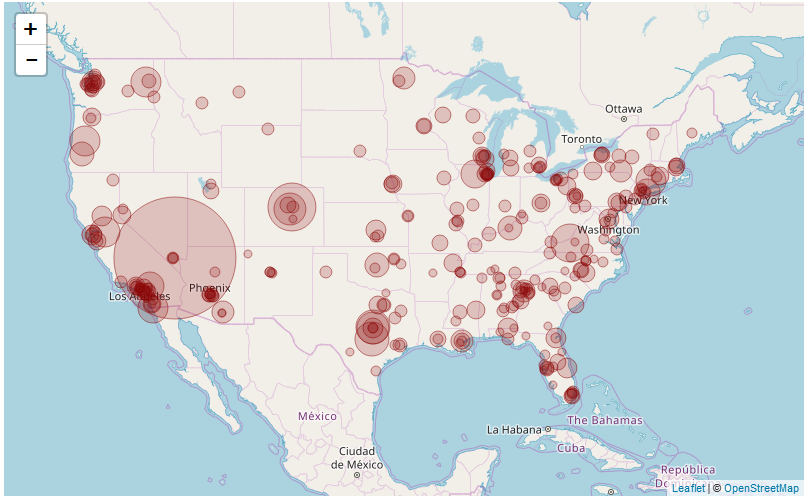
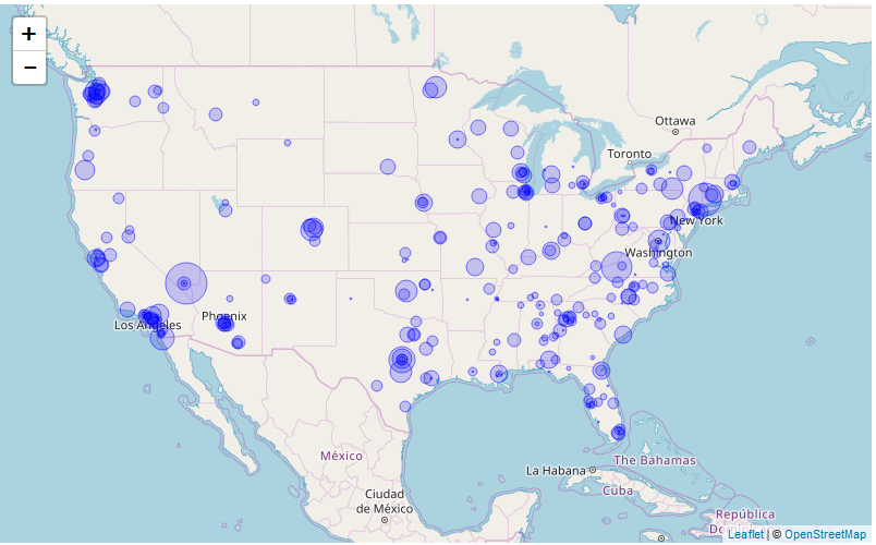
　　　　　　　　　　　　受伤人数分布　　　　　　　　　　　　　　　　　　　　　　　　　　　　　　　　　　　　死亡人数分布

　　结论:从地理信息结合人口信息来看,美国东部发生枪击案的概率要高于美国西部

　　4.3 枪手的性别分布

shooting %>%
  ggplot(aes(x=factor(Gender),fill=factor(Gender)))+
  geom_bar()+
  xlab('Gender')+
  ylab('Number of each Gender')+
  ggtitle('The distribution of gender')

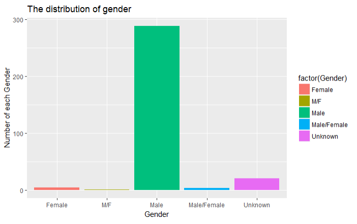
　　结论:男性作案的可能性远远大于女性

　　4.4 枪击案的种族分布

shooting %>% 
  na.omit() %>%
  group_by(Race) %>%
  summarise(num=sum(Total.victims)) %>%
  ggplot(aes(x=factor(Race),y=num,fill=factor(Race)))+
  geom_bar(stat = 'identity')+
  coord_polar(theta = 'y')+
  labs(x='Race',y='Number of killed people',fill='Race')+
  ggtitle('People killed by different race')

　　结论:白人作案很多,但是黑人作案的数量也在上升

　　4.5 枪击案的月份分布

shooting %>%
  mutate(month=month(Date)) %>%
  group_by(month) %>%
  summarise(n=sum(Total.victims)) %>%
  ggplot(aes(x=factor(month),y=n)) +
  geom_bar(stat = 'identity')+
  labs(x='month',y='Number of killed people')+
  ggtitle('The distribution of killed people every month')+
  geom_text(aes(label=n),vjust=-0.2,color='red')+
  theme_bw()

　　结论:10月份发生枪击案的数量最高,最危险

　　4.5 枪手是否有精神疾病

shooting %>% 
  na.omit() %>% 
  ggplot(aes(x=Mental.Health.Issues)) + 
  geom_bar()+
  scale_x_discrete(limits=c("NO","YES"))+
  theme_bw()

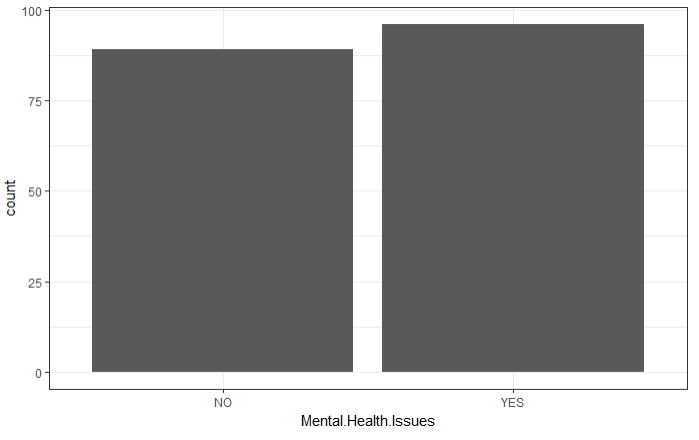
　　结论:凶手是否患有精神疾病并不是一个主要原因

　　4.6 患有精神疾病的和没有患有精神疾病的人是否是数量的差异

shooting %>%
  na.omit() %>%
  group_by(Mental.Health.Issues) %>%
  summarise(n=sum(Total.victims)) %>%
  ggplot(aes(x=factor(Mental.Health.Issues),y=n,group=1)) +
  geom_bar(stat = 'identity',fill='pink')+
  scale_x_discrete(limits=c('NO','YES'))+
  geom_text(aes(label=n),vjust=-0.2)+
  geom_line(color='red')

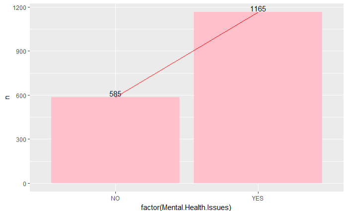
　　结论:患有精神疾病的凶手杀人的数量是没患有精神病人的一倍,精神病枪手的危害更大

　　4.7不同的时间段内,枪手种族的统计

shooting %>%
  na.omit() %>%
  group_by(yearcut) %>%
  ggplot(aes(x=yearcut,fill=Race))+
  geom_bar(position = 'dodge')

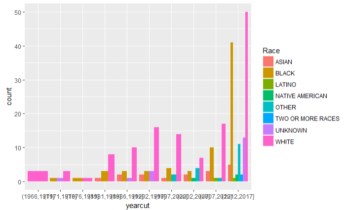
　　结论:可以看出虽然枪击案是以白人为主,但是在近几年来黑人翻案的数量也在不断增多

　　4.8枪手的年龄分布

# 通过正则表达式从摘要中提取年龄
tmp <- mutate(shooting,age=str_extract_all(shooting$Summary,pattern = '(,\s)\d{2}(,)'),
              age2 = str_extract_all(shooting$Summary,pattern = '(a\s)\d{2}(-year)'))
tmp$age <- str_sub(tmp$age,3,4)
tmp$age2 <- str_sub(tmp$age2,3,4)
# 去掉年龄不明的字段
te <- subset(tmp,tmp$age != 'ar')
te2 <- subset(tmp,tmp$age2 != 'ar')
te <- rbind(te,te2)

for(i in 1:nrow(te)){
  if(te$age[i] == 'ar'){
    te$age[i] = te$age2[i]
  }
}
te <- arrange(te,age)
te <- te[-c(1:4),]
te <- arrange(te,S.)
te$age <- as.integer(te$age)
te3 <- te %>%
  select(S.,age) %>%
  mutate(agecut=cut(te$age,breaks = 10*(1:7)))
shoot_age <- left_join(te3,shooting)

ggplot(data=shoot_age,aes(x=agecut))+
  geom_bar(fill='blue')+
  theme_bw()

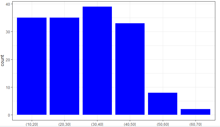
　　结论:从年龄分布上来看,年轻人作案的几率较大,冲动是魔鬼

　　4.9 不同年龄段精神疾病的分布

ggplot(data=shoot_age,aes(x=agecut,fill=Mental.Health.Issues))+
  geom_bar()

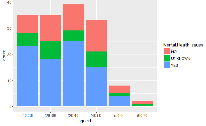
　　结论:10~20,和30~40岁之间的枪手群是精神疾病的高发群体

4.10 枪击案件的城市分布和州分布

# 城市分布
shooting %>%
  group_by(city) %>%
  summarise(count=n()) %>%
  filter(city != '' & count >= 2) %>%
  ggplot(aes(x=reorder(city,count),y=count))+
  geom_bar(stat = 'identity',fill='lightblue')+
  coord_flip()+
  labs(x='City',y='Number of gun-shot happended')+
  ggtitle('The number of case happened in each city')

# 州分布
shooting %>%
  group_by(state) %>%
  summarise(count=n()) %>%
  filter(state != '' & count >= 2) %>%
  ggplot(aes(reorder(state,count),y=count))+
  geom_bar(stat='identity',fill='lightblue')+
  coord_flip()+
  labs(x='State',y='Number of gun-shot happended')+
  ggtitle('The number of case happened in each state')

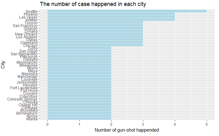
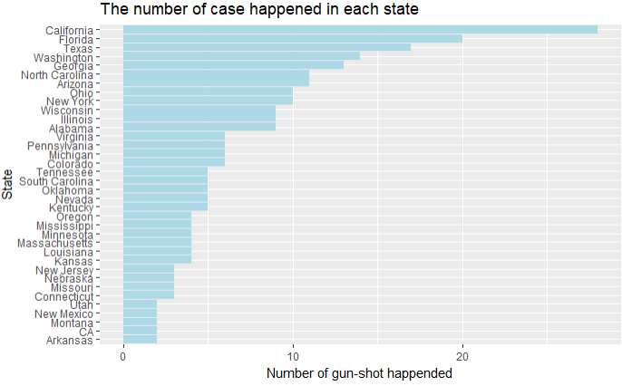
　　　　　　　　　　　　　　　　　　城市分布州分布

　　结论:发生枪击案件最多的是加州

总结:

　　1.从枪手的性别来看,男性作案是极大多数

　　2.从枪手的种族来看,白人是作案的主体,但是黑人作案的数量也在逐年上升

　　3.从枪手的年龄分布来看10~50岁之间的青中年占了绝大多数

　　4.从枪手的精神疾病来看,虽然枪手患有精神疾病和没有患有精神疾病的数量并不显著,但是患有精神疾病的枪手会造成更大的伤害,一定要重点控制

　　5.从枪击案件的时间上来看,枪支犯罪在2015年上升的最多,但是到了2017年有了一个极端的上升,可见控枪的重要性

　　6.从枪支案件的地理信息来看,总体上东部发生枪击案件的数量要大于西部

　　7.从枪击案发生的数量上来看,加州这几年发生枪击案的数量最多

代码:https://github.com/Mounment/R-Project