一、numpy库与matplotlib库的基本介绍
1.安装
(1)通过pip安装:
>> pip install matplotlib

安装完成
安装matplotlib的方式和numpy很像,下面不再介绍。
2.作用
(1)numpy:科学计算包,支持N维数组运算、处理大型矩阵、成熟的广播函数库、矢量运算、线性代数、傅里叶变换、随机数生成,并可与C++/Fortran语言无缝结合。树莓派Python v3默认安装已经包含了numpy。
numPy 是一个运行速度非常快的数学库,主要用于数组计算,包含:
- 一个强大的N维数组对象 ndarray
- 广播功能函数
- 整合 C/C++/Fortran 代码的工具
- 线性代数、傅里叶变换、随机数生成等功能
(2)
matplotlib: 可能是 Python 2D-绘图领域使用最广泛的套件。它能让使用者很轻松地将数据图形化,可以绘制多种形式的图形,包括线图、直方图、饼状图、散点图、误差线图等等并且提供多样化的输出格式。是数据可视化的重要工具。
二、扩展库numpy的简介
导入模块 >>> import numpy as np
生成数组
>>> np.array([1, 2, 3, 4, 5])        # 把列表转换为数组
array([1, 2, 3, 4, 5])
>>> np.array((1, 2, 3, 4, 5))        # 把元组转换成数组
array([1, 2, 3, 4, 5])
>>> np.array(range(5))               # 把range对象转换成数组
array([0, 1, 2, 3, 4])
>>> np.array([[1, 2, 3], [4, 5, 6]]) # 二维数组
array([[1, 2, 3],
       [4, 5, 6]])
>>> np.arange(8)                     # 类似于内置函数range()
array([0, 1, 2, 3, 4, 5, 6, 7])
>>> np.arange(1, 10, 2)
array([1, 3, 5, 7, 9])
生成各种各样的矩阵或数组,下面不再介绍
数组与数值的运算

>>> x = np.array((1, 2, 3, 4, 5))    # 创建数组对象
>>> x
array([1, 2, 3, 4, 5])
>>> x * 2                            # 数组与数值相乘,返回新数组
array([ 2, 4, 6, 8, 10])
>>> x / 2                            # 数组与数值相除
array([ 0.5, 1. , 1.5, 2. , 2.5])
>>> x // 2                           # 数组与数值整除
array([0, 1, 1, 2, 2], dtype=int32)
>>> x ** 3                           # 幂运算
array([1, 8, 27, 64, 125], dtype=int32)
>>> x + 2                            # 数组与数值相加
array([3, 4, 5, 6, 7])
>>> x % 3                            # 余数
array([1, 2, 0, 1, 2], dtype=int32)
>>> 2 ** x
array([2, 4, 8, 16, 32], dtype=int32)
>>> 2 / x
array([2. ,1. ,0.66666667, 0.5, 0.4])
>>> 63 // x
array([63, 31, 21, 15, 12], dtype=int32)
数组与数组的运算

>>> a = np.array((1, 2, 3))
>>> b = np.array(([1, 2, 3], [4, 5, 6], [7, 8, 9]))
>>> c = a * b                   # 数组与数组相乘
>>> c                           # a中的每个元素乘以b中的对应列元素
array([[ 1, 4, 9],
       [ 4, 10, 18],
       [ 7, 16, 27]])
>>> c / b                       # 数组之间的除法运算
array([[ 1.,  2.,  3.],
       [ 1.,  2.,  3.],
       [ 1.,  2.,  3.]])
>>> c / a
array([[ 1.,  2.,  3.],
       [ 4.,  5.,  6.],
       [ 7.,  8.,  9.]])
>>> a + a                         # 数组之间的加法运算
array([2, 4, 6])
>>> a * a                         # 数组之间的乘法运算
array([1, 4, 9])
>>> a - a                         # 数组之间的减法运算
array([0, 0, 0])
>>> a / a                         # 数组之间的除法运算
array([ 1.,  1.,  1.])
转置
>>> b = np.array(([1, 2, 3], [4, 5, 6], [7, 8, 9]))
>>> b
array([[1, 2, 3],
       [4, 5, 6],
       [7, 8, 9]])
>>> b.T                           # 转置
array([[1, 4, 7],
       [2, 5, 8],
       [3, 6, 9]])
参考资料:http://www.runoob.com/numpy/numpy-matplotlib.html
三、matplotlib库的简介
matplotlib中最基础的模块是pyplot
因为matplotlib库源于matlab,其操作基本如matlab的操作,以下用绘制一个函数的例子介绍matplotlib库。
import numpy as np
import matplotlib.pyplot as plt

X = np.linspace(-np.pi, np.pi, 256, endpoint=True)
C,S = np.cos(X), np.sin(X)

plt.plot(X,C)
plt.plot(X,S)

plt.show()
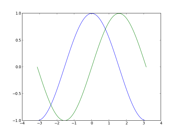
效果如下。
参考资料:http://www.runoob.com/w3cnote/matplotlib-tutorial.html
四、绘制雷达图
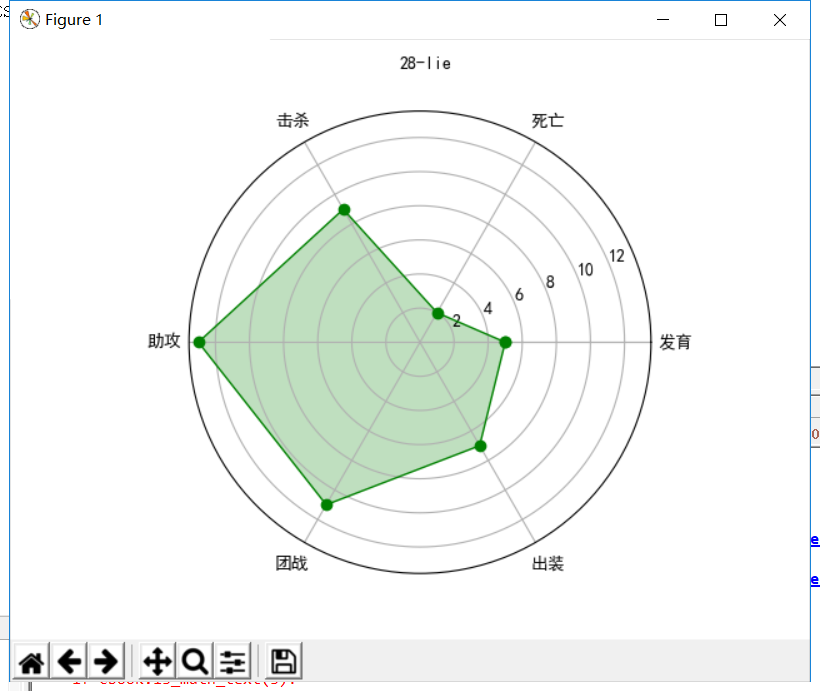
代码实现:
import numpy as np
import matplotlib.pyplot as plt
plt.rcParams['font.family'] = 'SimHei'        # 设置字体
plt.rcParams['font.sans-serif'] = ['SimHei']  # 设置字体

labels = np.array(['发育','死亡','击杀','助攻','团战','出装']) # 设置标签
datas = np.array([5, 2, 9, 13, 11, 7])       # 设置数据
angles = np.linspace(0, 2*np.pi, 6, endpoint = False) # 设置角度
datas = np.concatenate((datas, [datas[0]]))
angles = np.concatenate((angles, [angles[0]]))
fig = plt.figure(facecolor = 'white')         # 创建绘图区域
plt.subplot(111, polar = True)                # 极坐标
plt.plot(angles, datas, 'bo-', color = 'g', linewidth = 1) # 画图
plt.fill(angles, datas, facecolor = 'g', alpha = 0.25)     # 填充
plt.thetagrids(angles*180/np.pi, labels)      # 设置极坐标的位置
plt.figtext(0.52, 0.95, '28-lie', ha = 'center') # 设置标题
plt.grid(True)   # 打开网格线
plt.show()       # 展示图片
 五、此处展示PIL制作手绘风格
1.手绘图像的基本思想是利用像素之间的梯度值重构每个像素值,为了体现光照效果,设计一个光源,建立光源对个点梯度值的影响函数,进而运算出新的像素值,从而体现边界点灰度变化,形成手绘效果。
2.代码实现
from PIL import Image
import numpy as np
vec_el = np.pi/2.2 # 光源的俯视角度,弧度值
vec_az = np.pi/4. # 光源的方位角度,弧度值
depth = 10. # (0-100)
im = Image.open(r'C:Users80939Desktop	iantan.jpg').convert('L')
a = np.asarray(im).astype('float')
grad = np.gradient(a) #取图像灰度的梯度值
grad_x, grad_y = grad #分别取横纵图像梯度值
grad_x = grad_x*depth/100.
grad_y = grad_y*depth/100.
dx = np.cos(vec_el)*np.cos(vec_az) #光源对x 轴的影响
dy = np.cos(vec_el)*np.sin(vec_az) #光源对y 轴的影响
dz = np.sin(vec_el) #光源对z 轴的影响
A = np.sqrt(grad_x**2 + grad_y**2 + 1.)
uni_x = grad_x/A
uni_y = grad_y/A
uni_z = 1./A
a2 = 255*(dx*uni_x + dy*uni_y + dz*uni_z) #光源归一化
a2 = a2.clip(0,255)
im2 = Image.fromarray(a2.astype('uint8')) #重构图像
im2.save(r'C:Users80939Desktop	iantan1.jpg')
3.效果对比
