1.使用imhist()函数求图片直方图的时候,如果是RGB彩色图,则要首先调用rgb2gray()函数将其转化为灰度图。
eg:


1 ImageData=imread('baby.jpg');
2 I=rgb2gray(ImageData );
3 figure(1);
4 subplot(2,1,1);
5 imshow(ImageData);
6 subplot(2,1,2);
7 imshow(I);
8 figure(2);
9 imhist(uint8(I) );
执行结果如下:

2.bar可以用作绘制条状图、stem()函数绘制杆状图、plot()函数用来绘制图像最常见。
{
linspace()函数:
令A=linspace(1,100) 回车:然后会看到结果生成的是1到100之间的整数,一共100个数字,我们可以看到默认情况下linspace(a1,a2) 是生成包括a1 a2在内的等差数组。
linspace(a1,a2,N) 此函数是用来生成a1与a2之间等距的数组,间距d=(a2-a1)/(N-1)。例如B=linspace(0,9,9)我们可以看到结果如下:
B =
0 1.1250 2.2500 3.3750 4.5000 5.6250 6.7500 7.8750 9.0000
因为间距d = 1.125=(9-0)/(9-1)。
}
{
stem()函数:
stem(horz, z, 'fill')中,'fill'参数用来指示杆状图的标记点的颜色和线条的颜色,fill指示默认的‘蓝色,实线,圆’。如果换成‘r--p’就变成了'红色,虚线,五角星形'。详细的参数表格见《数字图像处理(MATLAB版)》P35。
}
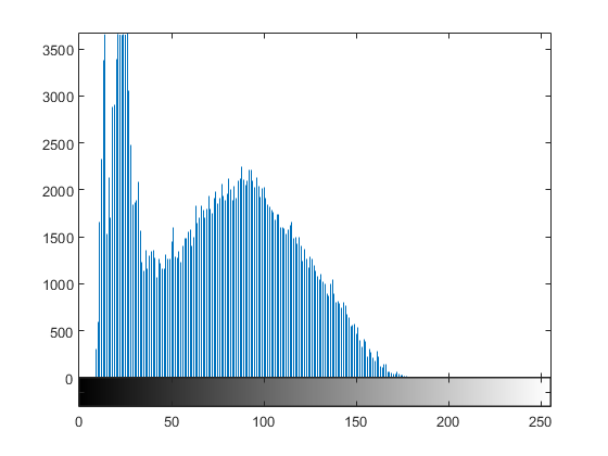
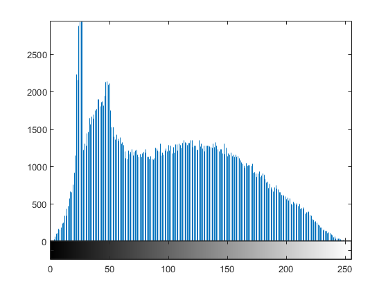
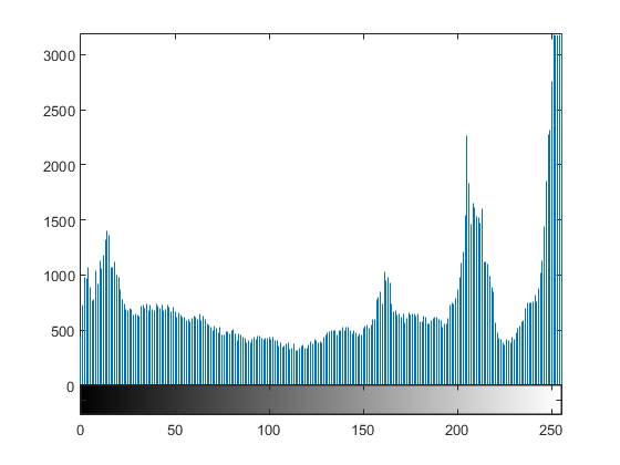
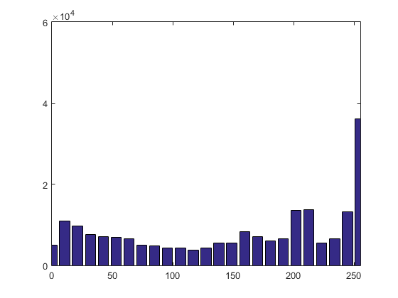
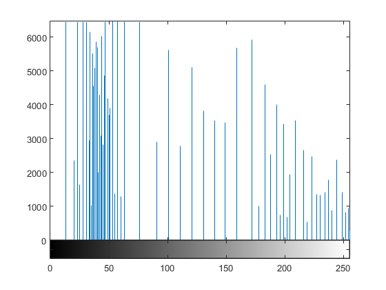
 1 ImageData=imread('baby.jpg');
 2 f=rgb2gray(ImageData );
 3 figure(1);
 4 imhist(f);                  %最原始的结果
 5
 6 figure(2);
 7 h = imhist(f,25);
 8 horz = linspace(0,255,25);
 9 bar(horz,h)                 %条形统计图
10 axis([0 255 0 60000] )
11 set(gca,'xtick',0:50:255)
12 set(gca,'ytick',0:20000:60000)
13
14 figure(3);
15 stem(horz,h,'fill');        %杆状图
16 axis([0 255 0 60000])
17 set(gca,'xtick',0:50:255)
18 set(gca,'ytick',0:20000:60000)
19
20 figure(4);
21 plot(imhist(f));
22 axis([0 255 0 15000])
23 set(gca,'xtick',0:50:255)
24 set(gca,'ytick',0:20000:60000)
结果如下图:


3.直方图均衡。g= histeq(f,nlev),f为输入图像,nlev为输出图像设定的灰度级数,默认为64。
 1 %{
 2 ImageData=imread('test.tif');
 3 f=rgb2gray(ImageData );
 4 %}
 5 clear,clc;
 6 close all;
 7 f = imread('test.tif');
 8 figure,imhist(f);                  %最原始的结果
 9 title('原图像直方图');
10 ylim('auto');
11 g = histeq(f,256);
12 figure,imshow(g)
13 title('均衡化处理后的图像');
14 figure,imhist(g)
15 title('均衡化后的直方图');
16 ylim('auto');
17
18 hnorm = imhist(f)./numel(f);
19 cdf = cumsum(hnorm);
20 x = linspace(0,1,256);
21 figure,plot(x,cdf);
22 title('变换函数');
23 axis([0 1 0 1]);
24 set(gca,'xtick',0:.2:1)
25 set(gca,'ytick',0:.2:1)
26 xlabel('Input intensity values','fontsize',9);
27 ylabel('Output intensity values','fontsize',9);
执行后结果为:


4.直方图规定化(自定义规定函数)
1 f = imread('test.tif'); %读入原图像
2 p = manualhist;         %输入规定直方图
3 g= histeq(f,p);         %调用histeq函数得到得到规定化直方图
4 figure,imhist(g);       %显示规定化后的直方图
如代码中所示,manualhist函数用来得到规定化直方图,并画出图像。 twomodegauss用来计算一个归一化到单位区域的双模态高斯函数。
manualhist函数为:
 1 function p = manualhist
 2 %MANUALHIST Generates a two-mode histogram interactively.
 3 %   P = MANUALHIST generates a two-mode histogram using
 4 %   TWOMODEGAUSS(m1, sig1, m2, sig2, A1, A2, k).  m1 and m2 are the
 5 %   means of the two modes and must be in the range [0,1].  sig1 and
 6 %   sig2 are the standard deviations of the two modes.  A1 and A2 are
 7 %   amplitude values, and k is an offset value that raised the
 8 %   "floor" of histogram.  The number of elements in the histogram
 9 %   vector P is 256 and sum(P) is normalized to 1.  MANUALHIST
10 %   repeatedly prompts for the parameters and plots the resulting
11 %   histogram until the user types an 'x' to quit, and then it returns
12 %   the last histogram computed.
13 %
14 %   A good set of starting values is: (0.15, 0.05, 0.75, 0.05, 1,
15 %   0.07, 0.002).
16
17 % Initialize.
18 repeats = true;
19 quitnow = 'x';
20
21 % Compute a default histogram in case the user quits before
22 % estimating at least one histogram.
23 p = twomodegauss(0.15, 0.05, 0.75, 0.05, 1, 0.07, 0.002);
24
25 % Cycle until an x is input.
26 while repeats
27    s = input('Enter m1, sig1, m2, sig2, A1, A2, k OR x to quit:','s');
28    if s == quitnow
29       break
30    end
31
32    % Convert the input string to a vector of numerical values and
33    % verify the number of inputs.
34    v = str2num(s);
35    if numel(v) ~= 7
36       disp('Incorrect number of inputs')
37       continue
38    end
39
40    p = twomodegauss(v(1), v(2), v(3), v(4), v(5), v(6), v(7));
41    % Start a new figure and scale the axes. Specifying only xlim
42    % leaves ylim on auto.
43    figure, plot(p)
44    xlim([0 255])
45 end
 1 function p = twomodegauss(m1, sig1, m2, sig2, A1, A2, k)
 2 %TWOMODEGAUSS Generates a two-mode Gaussian function.
 3 %   P = TWOMODEGAUSS(M1, SIG1, M2, SIG2, A1, A2, K) generates a
 4 %   two-mode, Gaussian-like function in the interval [0,1].  P is a
 5 %   256-element vector normalized so that SUM(P) equals 1.  The mean
 6 %   and standard deviation of the modes are (M1, SIG1) and (M2,
 7 %   SIG2), respectively. A1 and A2 are the amplitude values of the
 8 %   two modes.  Since the output is normalized, only the relative
 9 %   values of A1 and A2 are important.  K is an offset value that
10 %   raises the "floor" of the function.  A good set of values to try
11 %   is M1=0.15, S1=0.05, M2=0.75, S2=0.05, A1=1, A2=0.07, and
12 %   K=0.002.
13
14 %   Copyright 2002-2004 R. C. Gonzalez, R. E. Woods, & S. L. Eddins
15 %   Digital Image Processing Using MATLAB, Prentice-Hall, 2004
16 %   $Revision: 1.6 $  $Date: 2003/10/13 00:54:47 $
17
18 c1 = A1 * (1 / ((2 * pi) ^ 0.5) * sig1);
19 k1 = 2 * (sig1 ^ 2);
20 c2 = A2 * (1 / ((2 * pi) ^ 0.5) * sig2);
21 k2 = 2 * (sig2 ^ 2);
22 z  = linspace(0, 1, 256);
23
24 p = k + c1 * exp(-((z - m1) .^ 2) ./ k1) + ...
25     c2 * exp(-((z - m2) .^ 2) ./ k2);
26 p = p ./ sum(p(:));
执行结果为:

5.函数adapthisteq():自适应直方图均衡,这种方法用直方图匹配的方法来逐个处理图像中的较小区域。然后用双线性内插的方法来逐个将相邻的小片组合起来,从而消除人工引入的边界。特别是在均匀灰度区域,可以限制对比度来避免放大噪声。adapthisteq的语法是g = adapthisteq(f,param1,val1,param2,val2,...);
eg:
 1 clear,clc;
 2 close all;
 3 f = imread('test.tif'); %读入原图像
 4 imhist(f);
 5
 6 g1 = adapthisteq(f);
 7 figure,imhist(g1);
 8
 9 g2 = adapthisteq(f,'NumTiles',[25,25], 'ClipLimit',0.05 );
10 figure,imhist(g2);
得到的结果如下:很明显,均衡化处理的结果越来越好: