大致总结一下学到的各个优化算法。
一、梯度下降法
函数的梯度表示了函数值增长速度最快的方向,那么与其相反的方向,就可看作函数减少速度最快的方向。
在深度学习中,当目标设定为求解目标函数的最小值时,只要朝梯度下降的方向前进,就可以不断逼近最优值。
梯度下降主要组成部分:
1、待优化函数f(x)
2、待优化函数的导数g(x)
3、变量x,用于保存优化过程中的参数值
4、变量x点处的梯度值:grad
5、变量step,沿梯度下降方向前进的步长,即学习率
假设优化目标函数为:f(x) = (x-1)^2,那么导数为f'(x) = g(x) = 2x - 2。我们可以直接看出最优值在x = 1处取得。
import numpy as np
import matplotlib.pyplot as plt


def f(x):
    return (x-1)**2


def g(x):
    return 2 * x -2


def gd(x_start, step, g):
    x_list = []
    y_list = []
    x = x_start
    for i in range(20):
        grad = g(x)
        x = x - step*grad #往梯度反方向更新,***重点***
        x_list.append(x)
        y_list.append(f(x))
        print('x = {:}. grad = {:}, y = {:}'.format(x, grad, f(x)))

        if grad < 1e-6:
            break;
    return x_list,y_list


x = np.linspace(-8,10,200)
y = f(x)
//初始点为 x = 10, step = 0.1
x_gd, y_gd = gd(10, 0.1, g)

plt.plot(x, y)
plt.plot(x_gd, y_gd, 'r.')
plt.savefig('gradient_descent.png')
plt.show()
输出结果:
x = 8.2. grad = 18, y = 51.83999999999999
x = 6.76. grad = 14.399999999999999, y = 33.1776
x = 5.608. grad = 11.52, y = 21.233663999999997
x = 4.6864. grad = 9.216, y = 13.58954496
x = 3.9491199999999997. grad = 7.3728, y = 8.697308774399998
x = 3.3592959999999996. grad = 5.8982399999999995, y = 5.5662776156159985
x = 2.8874367999999997. grad = 4.718591999999999, y = 3.562417673994239
x = 2.5099494399999998. grad = 3.7748735999999994, y = 2.2799473113563127
x = 2.2079595519999997. grad = 3.0198988799999995, y = 1.45916627926804
x = 1.9663676415999998. grad = 2.4159191039999994, y = 0.9338664187315456
x = 1.7730941132799998. grad = 1.9327352831999995, y = 0.5976745079881891
x = 1.6184752906239999. grad = 1.5461882265599995, y = 0.3825116851124411
x = 1.4947802324992. grad = 1.2369505812479997, y = 0.2448074784719623
x = 1.3958241859993599. grad = 0.9895604649983998, y = 0.15667678622205583
x = 1.316659348799488. grad = 0.7916483719987197, y = 0.10027314318211579
x = 1.2533274790395903. grad = 0.633318697598976, y = 0.06417481163655406
x = 1.2026619832316723. grad = 0.5066549580791806, y = 0.04107187944739462
x = 1.1621295865853378. grad = 0.40532396646334456, y = 0.026286002846332555
x = 1.1297036692682703. grad = 0.32425917317067565, y = 0.016823041821652836
x = 1.1037629354146161. grad = 0.2594073385365405, y = 0.010766746765857796

二、Momentum动量算法
其实本质和梯度下降差不多,只是在更新梯度时,在原有梯度下降法的基础上,会将上一次的梯度乘上一个衰减率(pre_grad * discount),加入到本次的梯度更新中。
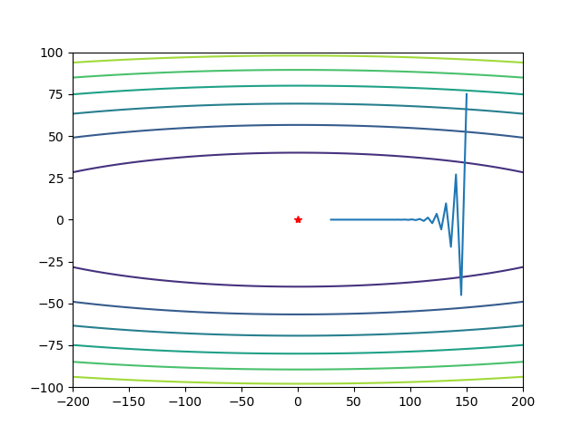
那么动量算法对比梯度下降法的好处在哪里呢?我们假设优化目标函数:z=x^2 + 50*y^2,那么使用梯度下降法的效果如何?请看:
import numpy as np
import matplotlib.pyplot as plt

def f(x):
    return x[0]*x[0] + 50*x[1]*x[1]


def g(x):
    return np.array([2*x[0], 100 * x[1]])


def gd(x_start, step, g):
    x_list = []
    y_list = []
    x = x_start
    x_list.append(x[0])
    y_list.append(x[1])
    for i in range(50):
        grad = g(x)
        x = x - step * grad
        print('ljj=',x)
        x_list.append(x[0])
        y_list.append(x[1])
        print('x = {:}. grad = {:}, y = {:}'.format(x, grad, f(x)))

        if grad.all() < 1e-6:
            break;
    return x_list, y_list


def momentum(x_start, step, g, discount = 0.7):
    x_list = []
    y_list = []
    x = x_start
    x_list.append(x[0])
    y_list.append(x[1])
    pre_grad = np.zeros_like(x)
    for i in range(50):
        grad = g(x)
        pre_grad = pre_grad * discount + step * grad  #将上一次更新量的乘上discount,再加上当前的梯度更新量。将结果用作本次更新
        x = x - pre_grad
        print('ljj=',x)
        x_list.append(x[0])
        y_list.append(x[1])
        print('x = {:}. grad = {:}, y = {:}'.format(x, grad, f(x)))

        if grad.all() < 1e-6:
            break;
    return x_list, y_list


xi = np.linspace(-200,200,1000)
yi = np.linspace(-100,100,1000)

X, Y = np.meshgrid(xi, yi)
Z = X*X + 50*Y*Y

#Gradient Descent
#xx,ss = gd([150, 75], 0.016, g)
#xx,ss = gd([150, 75], 0.019, g)

#Momentum
xx,ss = momentum([150, 75], 0.019, g)

print('xx=',xx)
print('xx=',xx[0])

plt.contour(X, Y, Z)
plt.plot(0,0, 'r*')
plt.plot(xx,ss)
plt.show()
梯度下降法【step = 0.016,迭代50次】:
梯度下降法【step = 0.019,迭代50次】:

动量算法【step = 0.019,迭代50次】:

从优化的路径来看,
梯度下降法,确实能够不断逼近最优值,但是由于存在冗余的Y方向上的更新,从而导致震荡明显,这些震荡有一部分是多余的开销。并且需要迭代次数较多,才能接近最优值。
动量算法,能够有效较少震荡,同时,加速优化,迭代次数相比梯度下降法更少,更快地逼近最优值。
三、Nesterov算法
在动量算法的基础上,再更进一步,计算梯度。--------简单来说,与动量算法的本质区别,只是在于计算梯度的区别:
1、动量算法:在当前目标点,计算梯度。
2、Nesterov:在当前目标的点基础上,再使用上次的梯度,进行一次动量更新,从而达到更新后的优化点。然后在此点上计算梯度。
def nesterov(x_start, step, g, discount = 0.7):
    x_list = []
    y_list = []
    x = x_start
    x_list.append(x[0])
    y_list.append(x[1])
    pre_grad = np.zeros_like(x)
    for i in range(50):
        x_future = x - pre_grad*step*discount  #使用上次的梯度,进行一次动量更新
        grad = g(x_future)             #在更新后的优化点上,计算梯度
        pre_grad = pre_grad * discount + grad
        x = x - pre_grad *step
        print('ljj=',x)
        x_list.append(x[0])
        y_list.append(x[1])
        print('x = {:}. grad = {:}, y = {:}'.format(x, grad, f(x)))

        if grad.all() < 1e-6:
            break;
    return x_list, y_list

xx,ss = nesterov([150, 75], 0.012, g)
结果如下:

通过调参(discount,step)可以看到,优化过程中,y轴方向的震荡明显快速减小。这就是Nesterov的效果。