Feature selection of sklearn

Feature selection

https://scikit-learn.org/stable/modules/feature_selection.html

     特征选择工具可以用于选择信息量大的特征，或者消减数据的维度， 以提高模型的精度， 或者提升模型在高维数据上的性能。

The classes in the sklearn.feature_selection module can be used for feature selection/dimensionality reduction on sample sets, either to improve estimators’ accuracy scores or to boost their performance on very high-dimensional datasets.

Removing features with low variance --- 变异度选择法

      VarianceThreshold 是一种简单的基线方法， 用于删除所有不符合门限值的特征。

     例如一个特征值是常量， 则没有任何信息量可言。

     低频变化的特征往往符合这种的特征。

VarianceThreshold is a simple baseline approach to feature selection. It removes all features whose variance doesn’t meet some threshold. By default, it removes all zero-variance features, i.e. features that have the same value in all samples.

As an example, suppose that we have a dataset with boolean features, and we want to remove all features that are either one or zero (on or off) in more than 80% of the samples. Boolean features are Bernoulli random variables, and the variance of such variables is given by

so we can select using the threshold .8 * (1 - .8):

>>> from sklearn.feature_selection import VarianceThreshold
>>> X = [[0, 0, 1], [0, 1, 0], [1, 0, 0], [0, 1, 1], [0, 1, 0], [0, 1, 1]]
>>> sel = VarianceThreshold(threshold=(.8 * (1 - .8)))
>>> sel.fit_transform(X)
array([[0, 1],
       [1, 0],
       [0, 0],
       [1, 1],
       [1, 0],
       [1, 1]])

VarianceThreshold

https://scikit-learn.org/stable/modules/generated/sklearn.feature_selection.VarianceThreshold.html#sklearn.feature_selection.VarianceThreshold

删除低变异特征。

Feature selector that removes all low-variance features.

This feature selection algorithm looks only at the features (X), not the desired outputs (y), and can thus be used for unsupervised learning.

>>> X = [[0, 2, 0, 3], [0, 1, 4, 3], [0, 1, 1, 3]]
>>> selector = VarianceThreshold()
>>> selector.fit_transform(X)
array([[2, 0],
       [1, 4],
       [1, 1]])

Univariate feature selection --- 单变量选择法

     使用单变量的统计测试方法， 卡方测试， F测试， 遴选出跟目标变量具有显著差异的变量。

Univariate feature selection works by selecting the best features based on univariate statistical tests. It can be seen as a preprocessing step to an estimator. Scikit-learn exposes feature selection routines as objects that implement the transform method:

• SelectKBest removes all but the

• highest scoring features

• SelectPercentile removes all but a user-specified highest scoring percentage of features

• using common univariate statistical tests for each feature: false positive rate SelectFpr, false discovery rate SelectFdr, or family wise error SelectFwe.

• GenericUnivariateSelect allows to perform univariate feature selection with a configurable strategy. This allows to select the best univariate selection strategy with hyper-parameter search estimator.

For instance, we can perform a

test to the samples to retrieve only the two best features as follows:

>>> from sklearn.datasets import load_iris
>>> from sklearn.feature_selection import SelectKBest
>>> from sklearn.feature_selection import chi2
>>> X, y = load_iris(return_X_y=True)
>>> X.shape
(150, 4)
>>> X_new = SelectKBest(chi2, k=2).fit_transform(X, y)
>>> X_new.shape
(150, 2)

检验选项：

These objects take as input a scoring function that returns univariate scores and p-values (or only scores for SelectKBest and SelectPercentile):

• For regression: f_regression, mutual_info_regression

• For classification: chi2, f_classif, mutual_info_classif

The methods based on F-test estimate the degree of linear dependency between two random variables. On the other hand, mutual information methods can capture any kind of statistical dependency, but being nonparametric, they require more samples for accurate estimation.

Univariate Feature Selection -- 示例

https://scikit-learn.org/stable/auto_examples/feature_selection/plot_feature_selection.html#sphx-glr-auto-examples-feature-selection-plot-feature-selection-py

对iris4个特征，添加20维度的噪音。

使用F检验选择最好的4个特征。

对比特征选择后的效果 和 未进行特征选择的效果， 包括SVM模型的对应特征的权值。

An example showing univariate feature selection.

Noisy (non informative) features are added to the iris data and univariate feature selection is applied. For each feature, we plot the p-values for the univariate feature selection and the corresponding weights of an SVM. We can see that univariate feature selection selects the informative features and that these have larger SVM weights.

In the total set of features, only the 4 first ones are significant. We can see that they have the highest score with univariate feature selection. The SVM assigns a large weight to one of these features, but also Selects many of the non-informative features. Applying univariate feature selection before the SVM increases the SVM weight attributed to the significant features, and will thus improve classification.

Out:

Classification accuracy without selecting features: 0.789
Classification accuracy after univariate feature selection: 0.868

 

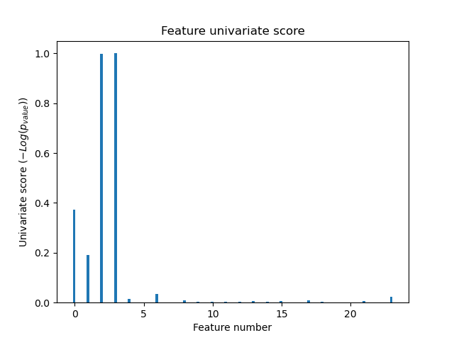
print(__doc__)

import numpy as np
import matplotlib.pyplot as plt

from sklearn.datasets import load_iris
from sklearn.model_selection import train_test_split
from sklearn.preprocessing import MinMaxScaler
from sklearn.svm import LinearSVC
from sklearn.pipeline import make_pipeline
from sklearn.feature_selection import SelectKBest, f_classif

# #############################################################################
# Import some data to play with

# The iris dataset
X, y = load_iris(return_X_y=True)

# Some noisy data not correlated
E = np.random.RandomState(42).uniform(0, 0.1, size=(X.shape[0], 20))

# Add the noisy data to the informative features
X = np.hstack((X, E))

# Split dataset to select feature and evaluate the classifier
X_train, X_test, y_train, y_test = train_test_split(
        X, y, stratify=y, random_state=0
)

plt.figure(1)
plt.clf()

X_indices = np.arange(X.shape[-1])

# #############################################################################
# Univariate feature selection with F-test for feature scoring
# We use the default selection function to select the four
# most significant features
selector = SelectKBest(f_classif, k=4)
selector.fit(X_train, y_train)
scores = -np.log10(selector.pvalues_)
scores /= scores.max()
plt.bar(X_indices - .45, scores, width=.2,
        label=r'Univariate score ($-Log(p_{value})$)')

# #############################################################################
# Compare to the weights of an SVM
clf = make_pipeline(MinMaxScaler(), LinearSVC())
clf.fit(X_train, y_train)
print('Classification accuracy without selecting features: {:.3f}'
      .format(clf.score(X_test, y_test)))

svm_weights = np.abs(clf[-1].coef_).sum(axis=0)
svm_weights /= svm_weights.sum()

plt.bar(X_indices - .25, svm_weights, width=.2, label='SVM weight')

clf_selected = make_pipeline(
        SelectKBest(f_classif, k=4), MinMaxScaler(), LinearSVC()
)
clf_selected.fit(X_train, y_train)
print('Classification accuracy after univariate feature selection: {:.3f}'
      .format(clf_selected.score(X_test, y_test)))

svm_weights_selected = np.abs(clf_selected[-1].coef_).sum(axis=0)
svm_weights_selected /= svm_weights_selected.sum()

plt.bar(X_indices[selector.get_support()] - .05, svm_weights_selected,
        width=.2, label='SVM weights after selection')


plt.title("Comparing feature selection")
plt.xlabel('Feature number')
plt.yticks(())
plt.axis('tight')
plt.legend(loc='upper right')
plt.show()

Comparison of F-test and mutual information -- 数据特性依赖

https://scikit-learn.org/stable/auto_examples/feature_selection/plot_f_test_vs_mi.html#sphx-glr-auto-examples-feature-selection-plot-f-test-vs-mi-py

F检验 更加适应于 数据具有线性特征。

mutual检验， 更加适合于 数据具有非线性特征。

毫无规律的数据， 则两种检验都不生效。

This example illustrates the differences between univariate F-test statistics and mutual information.

We consider 3 features x_1, x_2, x_3 distributed uniformly over [0, 1], the target depends on them as follows:

y = x_1 + sin(6 * pi * x_2) + 0.1 * N(0, 1), that is the third features is completely irrelevant.

The code below plots the dependency of y against individual x_i and normalized values of univariate F-tests statistics and mutual information.

As F-test captures only linear dependency, it rates x_1 as the most discriminative feature. On the other hand, mutual information can capture any kind of dependency between variables and it rates x_2 as the most discriminative feature, which probably agrees better with our intuitive perception for this example. Both methods correctly marks x_3 as irrelevant.

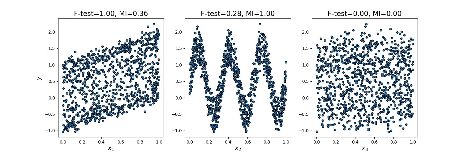
print(__doc__)

import numpy as np
import matplotlib.pyplot as plt
from sklearn.feature_selection import f_regression, mutual_info_regression

np.random.seed(0)
X = np.random.rand(1000, 3)
y = X[:, 0] + np.sin(6 * np.pi * X[:, 1]) + 0.1 * np.random.randn(1000)

f_test, _ = f_regression(X, y)
f_test /= np.max(f_test)

mi = mutual_info_regression(X, y)
mi /= np.max(mi)

plt.figure(figsize=(15, 5))
for i in range(3):
    plt.subplot(1, 3, i + 1)
    plt.scatter(X[:, i], y, edgecolor='black', s=20)
    plt.xlabel("$x_{}$".format(i + 1), fontsize=14)
    if i == 0:
        plt.ylabel("$y$", fontsize=14)
    plt.title("F-test={:.2f}, MI={:.2f}".format(f_test[i], mi[i]),
              fontsize=16)
plt.show()

Feature selection using SelectFromModel ---- 基于模型选择法

以上方法，均是基于特征数据本身， 但是对于模型来说对特征的评价，跟数据本身的特征还是有出入， 本方法思路是基于模型本身对特征的评价，来选择特征。

这种方法比较耗时， 需要在特征选择阶段就训练模型。

SelectFromModel is a meta-transformer that can be used along with any estimator that importance of each feature through a specific attribute (such as coef_, feature_importances_) or callable after fitting. The features are considered unimportant and removed, if the corresponding importance of the feature values are below the provided threshold parameter. Apart from specifying the threshold numerically, there are built-in heuristics for finding a threshold using a string argument. Available heuristics are “mean”, “median” and float multiples of these like “0.1*mean”. In combination with the threshold criteria, one can use the max_features parameter to set a limit on the number of features to select.

For examples on how it is to be used refer to the sections below.

L1-based feature selection

基于L1正则的特征选择。

线性模型带有L1正则惩罚项目， 会将相关度较小的特征系数极小化为0， 从而保留真正相关度较大的特征。

Linear models penalized with the L1 norm have sparse solutions: many of their estimated coefficients are zero. When the goal is to reduce the dimensionality of the data to use with another classifier, they can be used along with SelectFromModel to select the non-zero coefficients. In particular, sparse estimators useful for this purpose are the Lasso for regression, and of LogisticRegression and LinearSVC for classification:

>>> from sklearn.svm import LinearSVC
>>> from sklearn.datasets import load_iris
>>> from sklearn.feature_selection import SelectFromModel
>>> X, y = load_iris(return_X_y=True)
>>> X.shape
(150, 4)
>>> lsvc = LinearSVC(C=0.01, penalty="l1", dual=False).fit(X, y)
>>> model = SelectFromModel(lsvc, prefit=True)
>>> X_new = model.transform(X)
>>> X_new.shape
(150, 3)

Tree-based feature selection

基于树的特征选择。

相比线性模型， 此方法对特征的判断更加稳健，避免过拟合， 其使用的森林的集成学习方法。

Tree-based estimators (see the sklearn.tree module and forest of trees in the sklearn.ensemble module) can be used to compute impurity-based feature importances, which in turn can be used to discard irrelevant features (when coupled with the SelectFromModel meta-transformer):

>>> from sklearn.ensemble import ExtraTreesClassifier
>>> from sklearn.datasets import load_iris
>>> from sklearn.feature_selection import SelectFromModel
>>> X, y = load_iris(return_X_y=True)
>>> X.shape
(150, 4)
>>> clf = ExtraTreesClassifier(n_estimators=50)
>>> clf = clf.fit(X, y)
>>> clf.feature_importances_  
array([ 0.04...,  0.05...,  0.4...,  0.4...])
>>> model = SelectFromModel(clf, prefit=True)
>>> X_new = model.transform(X)
>>> X_new.shape               
(150, 2)

ExtraTreesClassifier

https://scikit-learn.org/stable/modules/generated/sklearn.ensemble.ExtraTreesClassifier.html#sklearn.ensemble.ExtraTreesClassifier

An extra-trees classifier.

This class implements a meta estimator that fits a number of randomized decision trees (a.k.a. extra-trees) on various sub-samples of the dataset and uses averaging to improve the predictive accuracy and control over-fitting.

>>> from sklearn.ensemble import ExtraTreesClassifier
>>> from sklearn.datasets import make_classification
>>> X, y = make_classification(n_features=4, random_state=0)
>>> clf = ExtraTreesClassifier(n_estimators=100, random_state=0)
>>> clf.fit(X, y)
ExtraTreesClassifier(random_state=0)
>>> clf.predict([[0, 0, 0, 0]])
array([1])

Feature importances with forests of trees

https://scikit-learn.org/stable/auto_examples/ensemble/plot_forest_importances.html#sphx-glr-auto-examples-ensemble-plot-forest-importances-py

树的森林对特征重要度的评价。

重要度为 模型给 对应特征的 打分。

This examples shows the use of forests of trees to evaluate the importance of features on an artificial classification task. The red bars are the impurity-based feature importances of the forest, along with their inter-trees variability.

As expected, the plot suggests that 3 features are informative, while the remaining are not.

Out:

Feature ranking:
1. feature 1 (0.295902)
2. feature 2 (0.208351)
3. feature 0 (0.177632)
4. feature 3 (0.047121)
5. feature 6 (0.046303)
6. feature 8 (0.046013)
7. feature 7 (0.045575)
8. feature 4 (0.044614)
9. feature 9 (0.044577)
10. feature 5 (0.043912)

 

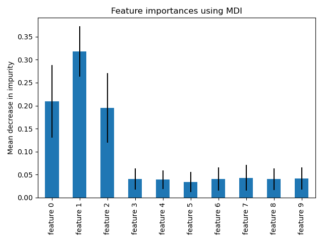
print(__doc__)

import numpy as np
import matplotlib.pyplot as plt

from sklearn.datasets import make_classification
from sklearn.ensemble import ExtraTreesClassifier

# Build a classification task using 3 informative features
X, y = make_classification(n_samples=1000,
                           n_features=10,
                           n_informative=3,
                           n_redundant=0,
                           n_repeated=0,
                           n_classes=2,
                           random_state=0,
                           shuffle=False)

# Build a forest and compute the impurity-based feature importances
forest = ExtraTreesClassifier(n_estimators=250,
                              random_state=0)

forest.fit(X, y)
importances = forest.feature_importances_
std = np.std([tree.feature_importances_ for tree in forest.estimators_],
             axis=0)
indices = np.argsort(importances)[::-1]

# Print the feature ranking
print("Feature ranking:")

for f in range(X.shape[1]):
    print("%d. feature %d (%f)" % (f + 1, indices[f], importances[indices[f]]))

# Plot the impurity-based feature importances of the forest
plt.figure()
plt.title("Feature importances")
plt.bar(range(X.shape[1]), importances[indices],
        color="r", yerr=std[indices], align="center")
plt.xticks(range(X.shape[1]), indices)
plt.xlim([-1, X.shape[1]])
plt.show()

Sequential Feature Selection

上面是基于特征的重要度进行选择。

另外一种思路是， 顺序依次添加特征， 或者顺序此减少特征。

Sequential Feature Selection [sfs] (SFS) is available in the SequentialFeatureSelector transformer. SFS can be either forward or backward:

Forward-SFS is a greedy procedure that iteratively finds the best new feature to add to the set of selected features. Concretely, we initially start with zero feature and find the one feature that maximizes a cross-validated score when an estimator is trained on this single feature. Once that first feature is selected, we repeat the procedure by adding a new feature to the set of selected features. The procedure stops when the desired number of selected features is reached, as determined by the n_features_to_select parameter.

Backward-SFS follows the same idea but works in the opposite direction: instead of starting with no feature and greedily adding features, we start with all the features and greedily remove features from the set. The direction parameter controls whether forward or backward SFS is used.

In general, forward and backward selection do not yield equivalent results. Also, one may be much faster than the other depending on the requested number of selected features: if we have 10 features and ask for 7 selected features, forward selection would need to perform 7 iterations while backward selection would only need to perform 3.

SFS differs from RFE and SelectFromModel in that it does not require the underlying model to expose a coef_ or feature_importances_ attribute. It may however be slower considering that more models need to be evaluated, compared to the other approaches. For example in backward selection, the iteration going from m features to m - 1 features using k-fold cross-validation requires fitting m * k models, while RFE would require only a single fit, and SelectFromModel always just does a single fit and requires no iterations.

Selecting features with Sequential Feature Selection

https://scikit-learn.org/stable/auto_examples/feature_selection/plot_select_from_model_diabetes.html#sphx-glr-auto-examples-feature-selection-plot-select-from-model-diabetes-py

Another way of selecting features is to use SequentialFeatureSelector (SFS). SFS is a greedy procedure where, at each iteration, we choose the best new feature to add to our selected features based a cross-validation score. That is, we start with 0 features and choose the best single feature with the highest score. The procedure is repeated until we reach the desired number of selected features.

We can also go in the reverse direction (backward SFS), i.e. start with all the features and greedily choose features to remove one by one. We illustrate both approaches here.

from sklearn.feature_selection import SequentialFeatureSelector

tic_fwd = time()
sfs_forward = SequentialFeatureSelector(lasso, n_features_to_select=2,
                                        direction='forward').fit(X, y)
toc_fwd = time()

tic_bwd = time()
sfs_backward = SequentialFeatureSelector(lasso, n_features_to_select=2,
                                         direction='backward').fit(X, y)
toc_bwd = time()

print("Features selected by forward sequential selection: "
      f"{feature_names[sfs_forward.get_support()]}")
print(f"Done in {toc_fwd - tic_fwd:.3f}s")
print("Features selected by backward sequential selection: "
      f"{feature_names[sfs_backward.get_support()]}")
print(f"Done in {toc_bwd - tic_bwd:.3f}s")

Feature selection as part of a pipeline

特征选择可以嵌入到 流水线中。

Feature selection is usually used as a pre-processing step before doing the actual learning. The recommended way to do this in scikit-learn is to use a Pipeline:

clf = Pipeline([
  ('feature_selection', SelectFromModel(LinearSVC(penalty="l1"))),
  ('classification', RandomForestClassifier())
])
clf.fit(X, y)

In this snippet we make use of a LinearSVC coupled with SelectFromModel to evaluate feature importances and select the most relevant features. Then, a RandomForestClassifier is trained on the transformed output, i.e. using only relevant features. You can perform similar operations with the other feature selection methods and also classifiers that provide a way to evaluate feature importances of course. See the Pipeline examples for more details.