Nearest Neighbors
https://scikit-learn.org/stable/modules/neighbors.html#nearest-neighbors-classification
sklearn.neighbors 提供了基于邻居的无监督和监督的学习方法。
无监督的最近邻是许多其他学习方法的基础, 著名的有 流形学习 和 谱聚类。
监督的基于邻居的学习有两种形式: 离散标签的分类算法, 连续型标签的回归算法。
最近邻方法的底层原理是 找出预定义数目的训练集样本, 这些样本是最接近于新的点, 并基于这些选出的样本预测它的标签。
样本点的数目有基于用户自定义常量(对应K近邻学习), 或者基于点的局部密度(基于半径的近邻学习)
sklearn.neighborsprovides functionality for unsupervised and supervised neighbors-based learning methods. Unsupervised nearest neighbors is the foundation of many other learning methods, notably manifold learning and spectral clustering. Supervised neighbors-based learning comes in two flavors: classification for data with discrete labels, and regression for data with continuous labels.The principle behind nearest neighbor methods is to find a predefined number of training samples closest in distance to the new point, and predict the label from these. The number of samples can be a user-defined constant (k-nearest neighbor learning), or vary based on the local density of points (radius-based neighbor learning). The distance can, in general, be any metric measure: standard Euclidean distance is the most common choice. Neighbors-based methods are known as non-generalizing machine learning methods, since they simply “remember” all of its training data (possibly transformed into a fast indexing structure such as a Ball Tree or KD Tree).
Despite its simplicity, nearest neighbors has been successful in a large number of classification and regression problems, including handwritten digits and satellite image scenes. Being a non-parametric method, it is often successful in classification situations where the decision boundary is very irregular.
The classes in
sklearn.neighborscan handle either NumPy arrays orscipy.sparsematrices as input. For dense matrices, a large number of possible distance metrics are supported. For sparse matrices, arbitrary Minkowski metrics are supported for searches.There are many learning routines which rely on nearest neighbors at their core. One example is kernel density estimation, discussed in the density estimation section.
Unsupervised Nearest Neighbors
NearestNeighbors 实现无监督的最近邻学习,实现了统一的接口对于三种不同的近邻学习算法(BallTree, KDTree, and a brute-force)。
NearestNeighborsimplements unsupervised nearest neighbors learning. It acts as a uniform interface to three different nearest neighbors algorithms:BallTree,KDTree, and a brute-force algorithm based on routines insklearn.metrics.pairwise. The choice of neighbors search algorithm is controlled through the keyword'algorithm', which must be one of['auto', 'ball_tree', 'kd_tree', 'brute']. When the default value'auto'is passed, the algorithm attempts to determine the best approach from the training data. For a discussion of the strengths and weaknesses of each option, see Nearest Neighbor Algorithms.For the simple task of finding the nearest neighbors between two sets of data, the unsupervised algorithms within
sklearn.neighborscan be used:
>>> from sklearn.neighbors import NearestNeighbors
>>> import numpy as np
>>> X = np.array([[-1, -1], [-2, -1], [-3, -2], [1, 1], [2, 1], [3, 2]])
>>> nbrs = NearestNeighbors(n_neighbors=2, algorithm='ball_tree').fit(X)
>>> distances, indices = nbrs.kneighbors(X)
>>> indices
array([[0, 1],
       [1, 0],
       [2, 1],
       [3, 4],
       [4, 3],
       [5, 4]]...)
>>> distances
array([[0.        , 1.        ],
       [0.        , 1.        ],
       [0.        , 1.41421356],
       [0.        , 1.        ],
       [0.        , 1.        ],
       [0.        , 1.41421356]])
查看最近邻的邻接矩阵。
Because the query set matches the training set, the nearest neighbor of each point is the point itself, at a distance of zero.
It is also possible to efficiently produce a sparse graph showing the connections between neighboring points:
>>> nbrs.kneighbors_graph(X).toarray()
array([[1., 1., 0., 0., 0., 0.],
       [1., 1., 0., 0., 0., 0.],
       [0., 1., 1., 0., 0., 0.],
       [0., 0., 0., 1., 1., 0.],
       [0., 0., 0., 1., 1., 0.],
       [0., 0., 0., 0., 1., 1.]])
对应的底层算法,也提供应用接口。
Alternatively, one can use the
KDTreeorBallTreeclasses directly to find nearest neighbors. This is the functionality wrapped by theNearestNeighborsclass used above. The Ball Tree and KD Tree have the same interface; we’ll show an example of using the KD Tree here:
>>> from sklearn.neighbors import KDTree
>>> import numpy as np
>>> X = np.array([[-1, -1], [-2, -1], [-3, -2], [1, 1], [2, 1], [3, 2]])
>>> kdt = KDTree(X, leaf_size=30, metric='euclidean')
>>> kdt.query(X, k=2, return_distance=False)
array([[0, 1],
       [1, 0],
       [2, 1],
       [3, 4],
       [4, 3],
       [5, 4]]...)
NearestNeighbors
https://scikit-learn.org/stable/modules/generated/sklearn.neighbors.NearestNeighbors.html#sklearn.neighbors.NearestNeighbors.kneighbors
Unsupervised learner for implementing neighbor searches.
    import numpy as np
    from sklearn.neighbors import NearestNeighbors
    samples = [[0, 0, 2], [1, 0, 0], [0, 0, 1]]

    >>>

    >>> neigh = NearestNeighbors(n_neighbors=2, radius=0.4)
    >>> neigh.fit(samples)
    NearestNeighbors(...)

    >>>

    >>> neigh.kneighbors([[0, 0, 1.3]], 2, return_distance=False)
    array([[2, 0]]...)

    >>>

    >>> nbrs = neigh.radius_neighbors(
    ...    [[0, 0, 1.3]], 0.4, return_distance=False
    ... )
    >>> np.asarray(nbrs[0][0])
    array(2)
KDTree
https://scikit-learn.org/stable/modules/generated/sklearn.neighbors.KDTree.html#sklearn.neighbors.KDTree
KDTree for fast generalized N-point problems
>>> import numpy as np
>>> rng = np.random.RandomState(0)
>>> X = rng.random_sample((10, 3))  # 10 points in 3 dimensions
>>> tree = KDTree(X, leaf_size=2)
>>> dist, ind = tree.query(X[:1], k=3)
>>> print(ind)  # indices of 3 closest neighbors
[0 3 1]
>>> print(dist)  # distances to 3 closest neighbors
[ 0.          0.19662693  0.29473397]
一文搞懂k近邻(k-NN)算法
https://zhuanlan.zhihu.com/p/25994179
k近邻算法是一种基本分类和回归方法。本篇文章只讨论分类问题的k近邻法。
K近邻算法,即是给定一个训练数据集,对新的输入实例,在训练数据集中找到与该实例最邻近的K个实例,这K个实例的多数属于某个类,就把该输入实例分类到这个类中。(这就类似于现实生活中少数服从多数的思想)根据这个说法,咱们来看下引自维基百科上的一幅图:
如上图所示,有两类不同的样本数据,分别用蓝色的小正方形和红色的小三角形表示,而图正中间的那个绿色的圆所标示的数据则是待分类的数据。这也就是我们的目的,来了一个新的数据点,我要得到它的类别是什么?好的,下面我们根据k近邻的思想来给绿色圆点进行分类。
- 如果K=3,绿色圆点的最邻近的3个点是2个红色小三角形和1个蓝色小正方形,少数从属于多数,基于统计的方法,判定绿色的这个待分类点属于红色的三角形一类。
- 如果K=5,绿色圆点的最邻近的5个邻居是2个红色三角形和3个蓝色的正方形,还是少数从属于多数,基于统计的方法,判定绿色的这个待分类点属于蓝色的正方形一类。
从上面例子我们可以看出,k近邻的算法思想非常的简单,也非常的容易理解,那么我们是不是就到此结束了,该算法的原理我们也已经懂了,也知道怎么给新来的点如何进行归类,只要找到离它最近的k个实例,哪个类别最多即可。
https://zhuanlan.zhihu.com/p/26029567
kd树原理
使用中值法切分样本空间,构造KD树。
对应树结构如下:

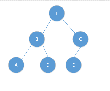
基于此树进行最近邻搜索。


Nearest Neighbors Classification
基于邻居的分类是一种 基于实例的学习, 或者是非泛化性学习。
不需要构造一个通用的内部模型, 仅仅是存储训练数据实例,分类是用过最近的邻居进行投票决定。
两种分类器:
KNeighborsClassifier 面向均匀分布
RadiusNeighborsClassifier 面向非均匀分布
可以设置权重, uniform 或者 distance, 前者将投票权设置为相同, 后者根据距离目标的距离设置权重。
Neighbors-based classification is a type of instance-based learning or non-generalizing learning: it does not attempt to construct a general internal model, but simply stores instances of the training data. Classification is computed from a simple majority vote of the nearest neighbors of each point: a query point is assigned the data class which has the most representatives within the nearest neighbors of the point.
scikit-learn implements two different nearest neighbors classifiers:
KNeighborsClassifierimplements learning based on thenearest neighbors of each query point, where is an integer value specified by the user.
RadiusNeighborsClassifierimplements learning based on the number of neighbors within a fixed radius of each training point, whereis a floating-point value specified by the user.
The-neighbors classification in
KNeighborsClassifieris the most commonly used technique. The optimal choice of the value is highly data-dependent: in general a largersuppresses the effects of noise, but makes the classification boundaries less distinct.
In cases where the data is not uniformly sampled, radius-based neighbors classification in
RadiusNeighborsClassifiercan be a better choice. The user specifies a fixed radius, such that points in sparser neighborhoods use fewer nearest neighbors for the classification. For high-dimensional parameter spaces, this method becomes less effective due to the so-called “curse of dimensionality”.
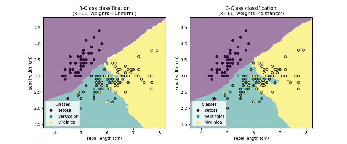
The basic nearest neighbors classification uses uniform weights: that is, the value assigned to a query point is computed from a simple majority vote of the nearest neighbors. Under some circumstances, it is better to weight the neighbors such that nearer neighbors contribute more to the fit. This can be accomplished through the
weightskeyword. The default value,weights = 'uniform', assigns uniform weights to each neighbor.weights = 'distance'assigns weights proportional to the inverse of the distance from the query point. Alternatively, a user-defined function of the distance can be supplied to compute the weights.
RadiusNeighborsClassifier
https://scikit-learn.org/stable/modules/generated/sklearn.neighbors.RadiusNeighborsClassifier.html#sklearn.neighbors.RadiusNeighborsClassifier
Classifier implementing a vote among neighbors within a given radius
>>> X = [[0], [1], [2], [3]]
>>> y = [0, 0, 1, 1]
>>> from sklearn.neighbors import RadiusNeighborsClassifier
>>> neigh = RadiusNeighborsClassifier(radius=1.0)
>>> neigh.fit(X, y)
RadiusNeighborsClassifier(...)
>>> print(neigh.predict([[1.5]]))
[0]
>>> print(neigh.predict_proba([[1.0]]))
[[0.66666667 0.33333333]]
Nearest Neighbors Classification -- 示例
https://scikit-learn.org/stable/auto_examples/neighbors/plot_classification.html#sphx-glr-auto-examples-neighbors-plot-classification-py
Sample usage of Nearest Neighbors classification. It will plot the decision boundaries for each class.

print(__doc__)

import numpy as np
import matplotlib.pyplot as plt
import seaborn as sns
from matplotlib.colors import ListedColormap
from sklearn import neighbors, datasets

n_neighbors = 15

# import some data to play with
iris = datasets.load_iris()

# we only take the first two features. We could avoid this ugly
# slicing by using a two-dim dataset
X = iris.data[:, :2]
y = iris.target

print("---------------- X ----------------")
print(X)

print("---------------- y ----------------")
print(y)


h = .02  # step size in the mesh

# Create color maps
cmap_light = ListedColormap(['orange', 'cyan', 'cornflowerblue'])
cmap_bold = ['darkorange', 'c', 'darkblue']

for weights in ['uniform', 'distance']:
    # we create an instance of Neighbours Classifier and fit the data.
    clf = neighbors.KNeighborsClassifier(n_neighbors, weights=weights)
    clf.fit(X, y)

    # Plot the decision boundary. For that, we will assign a color to each
    # point in the mesh [x_min, x_max]x[y_min, y_max].
    x_min, x_max = X[:, 0].min() - 1, X[:, 0].max() + 1
    y_min, y_max = X[:, 1].min() - 1, X[:, 1].max() + 1
    xx, yy = np.meshgrid(np.arange(x_min, x_max, h),
                         np.arange(y_min, y_max, h))

    print("---------------- xx.shape ----------------")
    print(xx.shape)

    print("---------------- yy.shape ----------------")
    print(yy.shape)

    Z = clf.predict(np.c_[xx.ravel(), yy.ravel()])

    print("---------------- Z.shape ----------------")
    print(Z.shape)

    # Put the result into a color plot
    Z = Z.reshape(xx.shape)

    print("---------------- Z.shape ----------------")
    print(Z.shape)


    plt.figure(figsize=(8, 6))
    plt.contourf(xx, yy, Z, cmap=cmap_light)

    # Plot also the training points
    sns.scatterplot(x=X[:, 0], y=X[:, 1], hue=iris.target_names[y],
                    palette=cmap_bold, alpha=1.0, edgecolor="black")

    plt.xlim(xx.min(), xx.max())
    plt.ylim(yy.min(), yy.max())

    plt.title("3-Class classification (k = %i, weights = '%s')"
              % (n_neighbors, weights))
    plt.xlabel(iris.feature_names[0])
    plt.ylabel(iris.feature_names[1])

plt.show()
Nearest Neighbors Regression
最近邻回归与分类相似, 只不过目标是 连续型数据, 最近邻投票的结果不是 类别,而是 几个最近邻目标的均值。
Neighbors-based regression can be used in cases where the data labels are continuous rather than discrete variables. The label assigned to a query point is computed based on the mean of the labels of its nearest neighbors.
scikit-learn implements two different neighbors regressors:
KNeighborsRegressorimplements learning based on thenearest neighbors of each query point, where is an integer value specified by the user.
RadiusNeighborsRegressorimplements learning based on the neighbors within a fixed radius of the query point, whereis a floating-point value specified by the user.
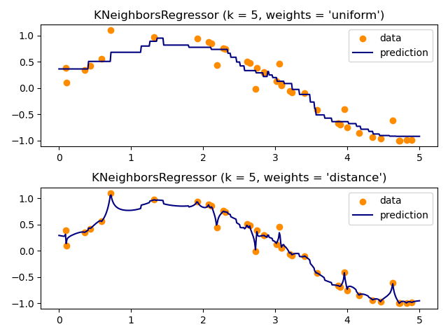
The basic nearest neighbors regression uses uniform weights: that is, each point in the local neighborhood contributes uniformly to the classification of a query point. Under some circumstances, it can be advantageous to weight points such that nearby points contribute more to the regression than faraway points. This can be accomplished through the
weightskeyword. The default value,weights = 'uniform', assigns equal weights to all points.weights = 'distance'assigns weights proportional to the inverse of the distance from the query point. Alternatively, a user-defined function of the distance can be supplied, which will be used to compute the weights.

Nearest Neighbors regression -- 示例
Demonstrate the resolution of a regression problem using a k-Nearest Neighbor and the interpolation of the target using both barycenter and constant weights.
print(__doc__)

# Author: Alexandre Gramfort <alexandre.gramfort@inria.fr>
#         Fabian Pedregosa <fabian.pedregosa@inria.fr>
#
# License: BSD 3 clause (C) INRIA


# #############################################################################
# Generate sample data
import numpy as np
import matplotlib.pyplot as plt
from sklearn import neighbors

np.random.seed(0)

base_X = np.random.rand(40, 1)

print("-------- base_X.shape ----------")
print(base_X.shape)


X = np.sort(5 * base_X, axis=0)

print("-------------- X.shape -----------------")
print(X.shape)

T = np.linspace(0, 5, 500)[:, np.newaxis]

print("-------------- T.shape -----------------")
print(T.shape)


y = np.sin(X).ravel()

print("-------------- y.shape -----------------")
print(y.shape)


# Add noise to targets
y[::5] += 1 * (0.5 - np.random.rand(8))


# #############################################################################
# Fit regression model
n_neighbors = 5

for i, weights in enumerate(['uniform', 'distance']):
    knn = neighbors.KNeighborsRegressor(n_neighbors, weights=weights)
    y_ = knn.fit(X, y).predict(T)

    plt.subplot(2, 1, i + 1)
    plt.scatter(X, y, color='darkorange', label='data')
    plt.plot(T, y_, color='navy', label='prediction')
    plt.axis('tight')
    plt.legend()
    plt.title("KNeighborsRegressor (k = %i, weights = '%s')" % (n_neighbors,
                                                                weights))

plt.tight_layout()
plt.show()