statistical learning -- Unsupervised learning of sklearn

Unsupervised learning

https://scikit-learn.org/stable/tutorial/statistical_inference/unsupervised_learning.html

      无监督学习的目的是， 寻找数据的表示。 探索数据的结构。

seeking representations of the data

Clustering: grouping observations together

    已知数据可以分为若干类， 但是并不知道数据属于哪一类， 可以使用聚类的方法进行探索。

The problem solved in clustering

Given the iris dataset, if we knew that there were 3 types of iris, but did not have access to a taxonomist to label them: we could try a clustering task: split the observations into well-separated group called clusters.

K-means clustering

https://scikit-learn.org/stable/tutorial/statistical_inference/unsupervised_learning.html#k-means-clustering

对于鸢尾花案例， 我们使用最简单的kmeans聚类方法。

Note that there exist a lot of different clustering criteria and associated algorithms. The simplest clustering algorithm is K-means.

>>>

从结果可知， 聚类之后，数据就有了标签。

在同一标签的下的数据，在原始数据中y的值也是相同的，也是一类数据。

>>> from sklearn import cluster, datasets
>>> X_iris, y_iris = datasets.load_iris(return_X_y=True)

>>> k_means = cluster.KMeans(n_clusters=3)
>>> k_means.fit(X_iris)
KMeans(n_clusters=3)
>>> print(k_means.labels_[::10])
[1 1 1 1 1 0 0 0 0 0 2 2 2 2 2]
>>> print(y_iris[::10])
[0 0 0 0 0 1 1 1 1 1 2 2 2 2 2]

但是聚类的结果往往没有稳定性保证， 很多事情不是确定的， 例如 聚类数目， 聚类初始化， 优化过程中容易掉入局部极小点。

所以不要过分解释聚类结果。

Warning

There is absolutely no guarantee of recovering a ground truth. First, choosing the right number of clusters is hard. Second, the algorithm is sensitive to initialization, and can fall into local minima, although scikit-learn employs several tricks to mitigate this issue.

 

Bad initialization

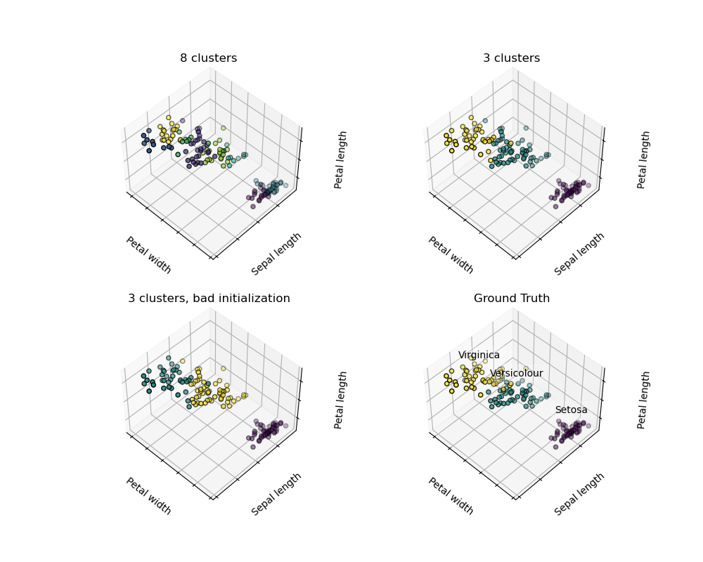
8 clusters

Ground truth

Don’t over-interpret clustering results

vector quantization

向量量化

聚类可以被看作是， 一种压缩数据信息的方法， 找到 一个更小的样本， 来代替原始的多样复杂的样本。

例如可以使用聚类来压缩图像。

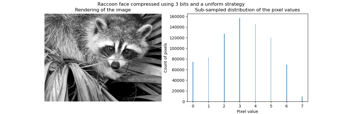
Clustering in general and KMeans, in particular, can be seen as a way of choosing a small number of exemplars to compress the information. The problem is sometimes known as vector quantization. For instance, this can be used to posterize an image:

>>> import scipy as sp
>>> try:
...    face = sp.face(gray=True)
... except AttributeError:
...    from scipy import misc
...    face = misc.face(gray=True)
>>> X = face.reshape((-1, 1)) # We need an (n_sample, n_feature) array
>>> k_means = cluster.KMeans(n_clusters=5, n_init=1)
>>> k_means.fit(X)
KMeans(n_clusters=5, n_init=1)
>>> values = k_means.cluster_centers_.squeeze()
>>> labels = k_means.labels_
>>> face_compressed = np.choose(labels, values)
>>> face_compressed.shape = face.shape

>>> face_compressed.shape = face.shape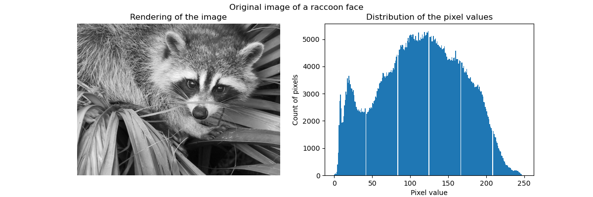

Raw image

K-means quantization

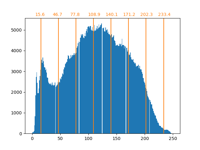
Equal bins

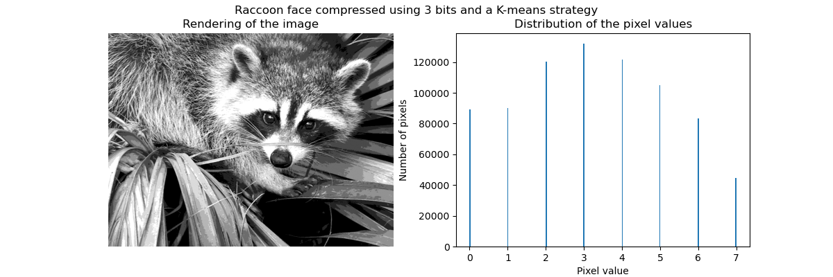
Image histogram

向量量化由来

https://en.wikipedia.org/wiki/Vector_quantization

向量量化是一种经典的信号处理领域的量化技术。

它允许使用原型向量的分布， 来建模概率分布函数 pdf。

最初被使用于数据压缩。

Vector quantization (VQ) is a classical quantization technique from signal processing that allows the modeling of probability density functions by the distribution of prototype vectors. It was originally used for data compression. It works by dividing a large set of points (vectors) into groups having approximately the same number of points closest to them. Each group is represented by its centroid point, as in k-means and some other clustering algorithms.

The density matching property of vector quantization is powerful, especially for identifying the density of large and high-dimensional data. Since data points are represented by the index of their closest centroid, commonly occurring data have low error, and rare data high error. This is why VQ is suitable for lossy data compression. It can also be used for lossy data correction and density estimation.

Vector quantization is based on the competitive learning paradigm, so it is closely related to the self-organizing map model and to sparse coding models used in deep learning algorithms such as autoencoder.

Hierarchical agglomerative clustering: Ward

https://scikit-learn.org/stable/tutorial/statistical_inference/unsupervised_learning.html#hierarchical-agglomerative-clustering-ward

于kmeans聚类不同， 层次聚类不用确定类的数目。

有两种聚类类型：

（1）聚合聚类 --- 从个体开始向群体演变

（2）分解聚类 -- 从初始的大群，演变成一个个的小群。

A Hierarchical clustering method is a type of cluster analysis that aims to build a hierarchy of clusters. In general, the various approaches of this technique are either:

• Agglomerative - bottom-up approaches: each observation starts in its own cluster, and clusters are iteratively merged in such a way to minimize a linkage criterion. This approach is particularly interesting when the clusters of interest are made of only a few observations. When the number of clusters is large, it is much more computationally efficient than k-means.

• Divisive - top-down approaches: all observations start in one cluster, which is iteratively split as one moves down the hierarchy. For estimating large numbers of clusters, this approach is both slow (due to all observations starting as one cluster, which it splits recursively) and statistically ill-posed.

 

Decompositions: from a signal to components and loadings

https://scikit-learn.org/stable/tutorial/statistical_inference/unsupervised_learning.html#decompositions-from-a-signal-to-components-and-loadings

分解， 从一个信号中分解为不同的成分， 和 荷载。

  信号    包含两个部分 成分 和 荷载。

  成分 可以理解为 高低频， 荷载为信号中有效信息。

Components and loadings

If X is our multivariate data, then the problem that we are trying to solve is to rewrite it on a different observational basis: we want to learn loadings L and a set of components C such that X = L C. Different criteria exist to choose the components

Principal component analysis: PCA

https://scikit-learn.org/stable/tutorial/statistical_inference/unsupervised_learning.html#principal-component-analysis-pca

主成分分析，会选择系列的成分， 这些成分可以最大化地解释信号。

Principal component analysis (PCA) selects the successive components that explain the maximum variance in the signal.

The point cloud spanned by the observations above is very flat in one direction: one of the three univariate features can almost be exactly computed using the other two. PCA finds the directions in which the data is not flat

When used to transform data, PCA can reduce the dimensionality of the data by projecting on a principal subspace.

三维数据， 通过PCA分析，降低为二维数据。

>>> # Create a signal with only 2 useful dimensions
>>> x1 = np.random.normal(size=100)
>>> x2 = np.random.normal(size=100)
>>> x3 = x1 + x2
>>> X = np.c_[x1, x2, x3]

>>> from sklearn import decomposition
>>> pca = decomposition.PCA()
>>> pca.fit(X)
PCA()
>>> print(pca.explained_variance_)  
[  2.18565811e+00   1.19346747e+00   8.43026679e-32]

>>> # As we can see, only the 2 first components are useful
>>> pca.n_components = 2
>>> X_reduced = pca.fit_transform(X)
>>> X_reduced.shape
(100, 2)

Independent Component Analysis: ICA

https://scikit-learn.org/stable/tutorial/statistical_inference/unsupervised_learning.html#independent-component-analysis-ica

独立成分分析， 选择这些成分， 他们负载分布携带最大量的独立信息。

Independent component analysis (ICA) selects components so that the distribution of their loadings carries a maximum amount of independent information. It is able to recover non-Gaussian independent signals:

>>> # Generate sample data
>>> import numpy as np
>>> from scipy import signal
>>> time = np.linspace(0, 10, 2000)
>>> s1 = np.sin(2 * time)  # Signal 1 : sinusoidal signal
>>> s2 = np.sign(np.sin(3 * time))  # Signal 2 : square signal
>>> s3 = signal.sawtooth(2 * np.pi * time)  # Signal 3: saw tooth signal
>>> S = np.c_[s1, s2, s3]
>>> S += 0.2 * np.random.normal(size=S.shape)  # Add noise
>>> S /= S.std(axis=0)  # Standardize data
>>> # Mix data
>>> A = np.array([[1, 1, 1], [0.5, 2, 1], [1.5, 1, 2]])  # Mixing matrix
>>> X = np.dot(S, A.T)  # Generate observations

>>> # Compute ICA
>>> ica = decomposition.FastICA()
>>> S_ = ica.fit_transform(X)  # Get the estimated sources
>>> A_ = ica.mixing_.T
>>> np.allclose(X,  np.dot(S_, A_) + ica.mean_)
True

Principal components analysis (PCA) -- 示例

https://scikit-learn.org/stable/auto_examples/decomposition/plot_pca_3d.html

These figures aid in illustrating how a point cloud can be very flat in one direction–which is where PCA comes in to choose a direction that is not flat.

• 
• 

print(__doc__)

# Authors: Gael Varoquaux
#          Jaques Grobler
#          Kevin Hughes
# License: BSD 3 clause

from sklearn.decomposition import PCA

from mpl_toolkits.mplot3d import Axes3D
import numpy as np
import matplotlib.pyplot as plt
from scipy import stats


# #############################################################################
# Create the data

e = np.exp(1)
np.random.seed(4)


def pdf(x):
    return 0.5 * (stats.norm(scale=0.25 / e).pdf(x)
                  + stats.norm(scale=4 / e).pdf(x))

y = np.random.normal(scale=0.5, size=(30000))
x = np.random.normal(scale=0.5, size=(30000))
z = np.random.normal(scale=0.1, size=len(x))

density = pdf(x) * pdf(y)
pdf_z = pdf(5 * z)

density *= pdf_z

a = x + y
b = 2 * y
c = a - b + z

norm = np.sqrt(a.var() + b.var())
a /= norm
b /= norm


# #############################################################################
# Plot the figures
def plot_figs(fig_num, elev, azim):
    fig = plt.figure(fig_num, figsize=(4, 3))
    plt.clf()
    ax = Axes3D(fig, rect=[0, 0, .95, 1], elev=elev, azim=azim)

    ax.scatter(a[::10], b[::10], c[::10], c=density[::10], marker='+', alpha=.4)
    Y = np.c_[a, b, c]

    # Using SciPy's SVD, this would be:
    # _, pca_score, Vt = scipy.linalg.svd(Y, full_matrices=False)

    pca = PCA(n_components=3)
    pca.fit(Y)
    V = pca.components_.T

    x_pca_axis, y_pca_axis, z_pca_axis = 3 * V
    x_pca_plane = np.r_[x_pca_axis[:2], - x_pca_axis[1::-1]]
    y_pca_plane = np.r_[y_pca_axis[:2], - y_pca_axis[1::-1]]
    z_pca_plane = np.r_[z_pca_axis[:2], - z_pca_axis[1::-1]]
    x_pca_plane.shape = (2, 2)
    y_pca_plane.shape = (2, 2)
    z_pca_plane.shape = (2, 2)
    ax.plot_surface(x_pca_plane, y_pca_plane, z_pca_plane)
    ax.w_xaxis.set_ticklabels([])
    ax.w_yaxis.set_ticklabels([])
    ax.w_zaxis.set_ticklabels([])


elev = -40
azim = -80
plot_figs(1, elev, azim)

elev = 30
azim = 20
plot_figs(2, elev, azim)

plt.show()

Blind source separation using FastICA 示例

https://scikit-learn.org/stable/auto_examples/decomposition/plot_ica_blind_source_separation.html

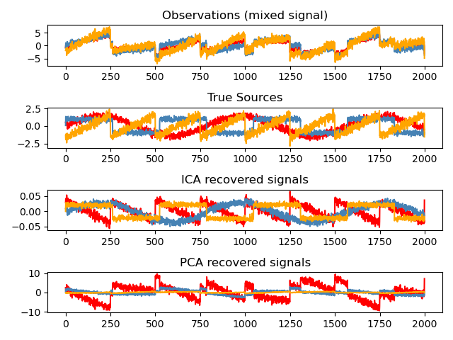
An example of estimating sources from noisy data.

Independent component analysis (ICA) is used to estimate sources given noisy measurements. Imagine 3 instruments playing simultaneously and 3 microphones recording the mixed signals. ICA is used to recover the sources ie. what is played by each instrument. Importantly, PCA fails at recovering our instruments since the related signals reflect non-Gaussian processes.

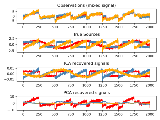
print(__doc__)

import numpy as np
import matplotlib.pyplot as plt
from scipy import signal

from sklearn.decomposition import FastICA, PCA

# #############################################################################
# Generate sample data
np.random.seed(0)
n_samples = 2000
time = np.linspace(0, 8, n_samples)

s1 = np.sin(2 * time)  # Signal 1 : sinusoidal signal
s2 = np.sign(np.sin(3 * time))  # Signal 2 : square signal
s3 = signal.sawtooth(2 * np.pi * time)  # Signal 3: saw tooth signal

S = np.c_[s1, s2, s3]
S += 0.2 * np.random.normal(size=S.shape)  # Add noise

S /= S.std(axis=0)  # Standardize data
# Mix data
A = np.array([[1, 1, 1], [0.5, 2, 1.0], [1.5, 1.0, 2.0]])  # Mixing matrix
X = np.dot(S, A.T)  # Generate observations

# Compute ICA
ica = FastICA(n_components=3)
S_ = ica.fit_transform(X)  # Reconstruct signals
A_ = ica.mixing_  # Get estimated mixing matrix

# We can `prove` that the ICA model applies by reverting the unmixing.
assert np.allclose(X, np.dot(S_, A_.T) + ica.mean_)

# For comparison, compute PCA
pca = PCA(n_components=3)
H = pca.fit_transform(X)  # Reconstruct signals based on orthogonal components

# #############################################################################
# Plot results

plt.figure()

models = [X, S, S_, H]
names = ['Observations (mixed signal)',
         'True Sources',
         'ICA recovered signals',
         'PCA recovered signals']
colors = ['red', 'steelblue', 'orange']

for ii, (model, name) in enumerate(zip(models, names), 1):
    plt.subplot(4, 1, ii)
    plt.title(name)
    for sig, color in zip(model.T, colors):
        plt.plot(sig, color=color)

plt.tight_layout()
plt.show()