一个复数序列可以分解为共轭偶对称和共轭奇对称部分。
代码:
%% ------------------------------------------------------------------------
%% Output Info about this m-file
fprintf('
***********************************************************
');
fprintf(' <DSP using MATLAB> Problem 3.7
');
banner();
%% ------------------------------------------------------------------------
n_start = -10; n_end = 20;
n = [n_start:n_end];
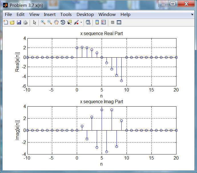
x = 2 * (0.9 .^(-n)) .* (cos(0.1*pi*n) + j*sin(0.9*pi*n)) .* (stepseq(0, n_start, n_end)-stepseq(10, n_start, n_end));
[xe,xo,m] = evenodd_cv(x,n);
figure('NumberTitle', 'off', 'Name', 'Problem 3.7 x(n)')
set(gcf,'Color',[1,1,1]) % 改变坐标外围背景颜色
subplot(2,1,1); stem(n, real(x)); title('x sequence Real Part');
xlabel('n'); ylabel('Real[x(n)]') ;
% axis([-10,10,0,1.2])
grid on
subplot(2,1,2); stem(n, imag(x)); title('x sequence Imag Part');
xlabel('n'); ylabel('Imag[x(n)]');
grid on;
figure('NumberTitle', 'off', 'Name', 'Problem 3.7 xe(m)')
set(gcf,'Color',[1,1,1])
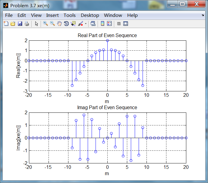
subplot(2,1,1); stem(m, real(xe)); title('Real Part of Even Sequence');
xlabel('m'); ylabel('Real[xe(m)]');
%axis([-10,10,0,1.2])
grid on
subplot(2,1,2); stem(m, imag(xe)); title('Imag Part of Even Sequence');
xlabel('m'); ylabel('Imag[xe(m)]');
%axis([-10,10,0,1.2])
grid on
figure('NumberTitle', 'off', 'Name', 'Problem 3.7 xo(m)')
set(gcf,'Color','white')
subplot(2,1,1); stem(m, real(xo)); title('Real Part of Odd Sequence');
xlabel('m'); ylabel('Real[xo(m)]');
%axis([-10,10,0,1.2])
grid on
subplot(2,1,2); stem(m, imag(xo)); title('Imag Part of Odd Sequence');
xlabel('m'); ylabel('Imag[xo(m)]');
%axis([-10,10,0,1.2])
grid on
% ----------------------------------------------
% DTFT of x(n)
% ----------------------------------------------
MM = 500;
k = [-MM:MM]; % [-pi, pi]
%k = [0:M]; % [0, pi]
w = (pi/MM) * k;
[X] = dtft(x, n, w);
magX = abs(X); angX = angle(X); realX = real(X); imagX = imag(X);
figure('NumberTitle', 'off', 'Name', 'Problem 3.7 DTFT of x(n)');
set(gcf,'Color','white');
subplot(2,1,1); plot(w/pi, magX); grid on;
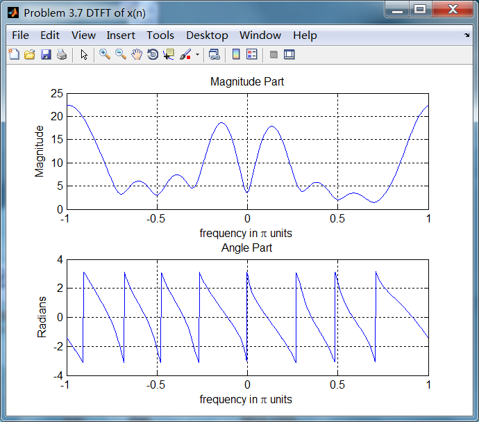
title('Magnitude Part');
xlabel('frequency in pi units'); ylabel('Magnitude');
subplot(2,1,2); plot(w/pi, angX); grid on;
title('Angle Part');
xlabel('frequency in pi units'); ylabel('Radians');
figure('NumberTitle', 'off', 'Name', 'Problem 3.7 Real and Imag of X(jw)');
set(gcf,'Color','white');
subplot('2,1,1'); plot(w/pi, realX); grid on;
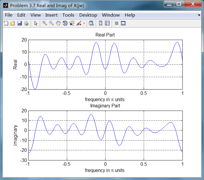
title('Real Part');
xlabel('frequency in pi units'); ylabel('Real');
subplot('2,1,2'); plot(w/pi, imagX); grid on;
title('Imaginary Part');
xlabel('frequency in pi units'); ylabel('Imaginary');
% ---------------------------------------------------
% DTFT of xe(m)
% ---------------------------------------------------
MM = 500;
k = [-MM:MM]; % [-pi, pi]
%k = [0:M]; % [0, pi]
w = (pi/MM) * k;
[XE] = dtft(xe, m, w);
magXE = abs(XE); angXE = angle(XE); realXE = real(XE); imagXE = imag(XE);
figure('NumberTitle', 'off', 'Name', 'Problem 3.7 DTFT of xe(m)');
set(gcf,'Color','white');
subplot(2,1,1); plot(w/pi, magXE); grid on;
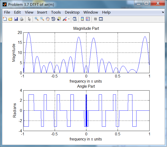
title('Magnitude Part');
xlabel('frequency in pi units'); ylabel('Magnitude');
subplot(2,1,2); plot(w/pi, angXE); grid on;
title('Angle Part');
xlabel('frequency in pi units'); ylabel('Radians');
figure('NumberTitle', 'off', 'Name', 'Problem 3.7 Real and Imag of XE(jw)');
set(gcf,'Color','white');
subplot('2,1,1'); plot(w/pi, realXE); grid on;
title('Real Part');
xlabel('frequency in pi units'); ylabel('Real');
subplot('2,1,2'); plot(w/pi, imagXE); grid on;
title('Imaginary Part');
xlabel('frequency in pi units'); ylabel('Imaginary');
% ---------------------------------------------------
% DTFT of xo(m)
% ---------------------------------------------------
MM = 500;
k = [-MM:MM]; % [-pi, pi]
%k = [0:M]; % [0, pi]
w = (pi/MM) * k;
[XO] = dtft(xo, m, w);
magXO = abs(XO); angXO = angle(XO); realXO = real(XO); imagXO = imag(XO);
figure('NumberTitle', 'off', 'Name', 'Problem 3.7 DTFT of xo(m)');
set(gcf,'Color','white');
subplot(2,1,1); plot(w/pi, magXO); grid on;
title('Magnitude Part');
xlabel('frequency in pi units'); ylabel('Magnitude');
subplot(2,1,2); plot(w/pi, angXO); grid on;
title('Angle Part');
xlabel('frequency in pi units'); ylabel('Radians');
figure('NumberTitle', 'off', 'Name', 'Problem 3.7 Real and Imag of XO(jw)');
set(gcf,'Color','white');
subplot('2,1,1'); plot(w/pi, realXO); grid on;
title('Real Part');
xlabel('frequency in pi units'); ylabel('Real');
subplot('2,1,2'); plot(w/pi, imagXO); grid on;
title('Imaginary Part');
xlabel('frequency in pi units'); ylabel('Imaginary');
% ------------------------------------------
% Verify
% ------------------------------------------
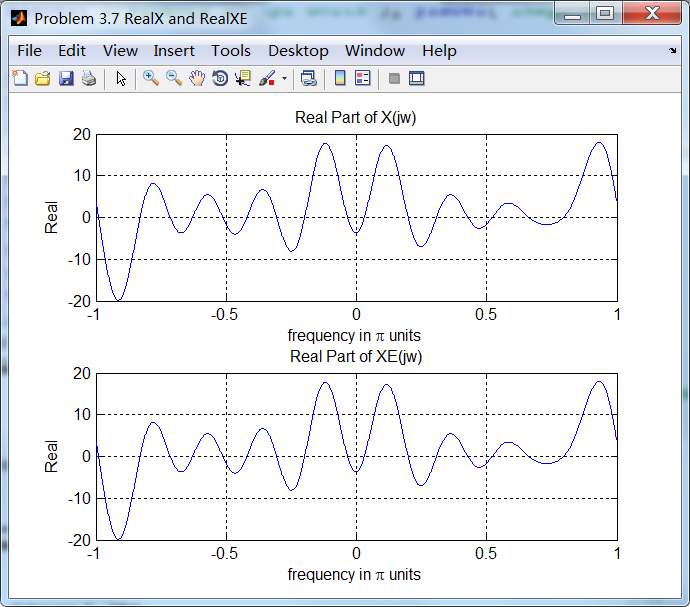
figure('NumberTitle', 'off', 'Name', 'Problem 3.7 RealX and RealXE');
set(gcf,'Color','white');
subplot('2,1,1'); plot(w/pi, realX); grid on;
title('Real Part of X(jw)');
xlabel('frequency in pi units'); ylabel('Real');
subplot('2,1,2'); plot(w/pi, realXE); grid on;
title('Real Part of XE(jw)');
xlabel('frequency in pi units'); ylabel('Real');
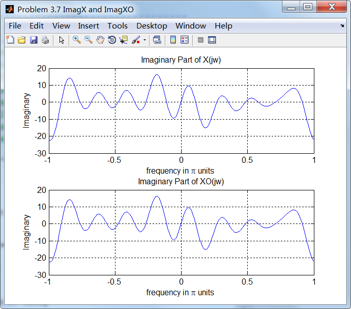
figure('NumberTitle', 'off', 'Name', 'Problem 3.7 ImagX and ImagXO');
set(gcf,'Color','white');
subplot('2,1,1'); plot(w/pi, imagX); grid on;
title('Imaginary Part of X(jw)');
xlabel('frequency in pi units'); ylabel('Imaginary');
subplot('2,1,2'); plot(w/pi, imagXO); grid on;
title('Imaginary Part of XO(jw)');
xlabel('frequency in pi units'); ylabel('Imaginary');
运行结果:
1、原始序列,及其共轭奇偶分解(都是复数序列);

2、原始序列的DTFT,幅度谱和相位谱,实部和虚部;
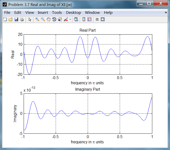
3、共轭偶(奇)对称序列的DTFT
4、共轭奇对称序列的DTFT
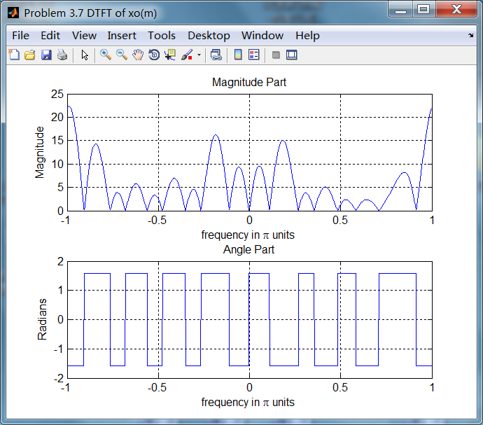
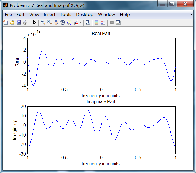
5、结论
原始序列谱的实部和共轭偶对称序列的谱相同;
原始序列谱的虚部和共轭奇对称序列的谱相同;