代码:
%% ++++++++++++++++++++++++++++++++++++++++++++++++++++++++++++++++++++++++++++++++
%% Output Info about this m-file
fprintf('
***********************************************************
');
fprintf(' <DSP using MATLAB> Problem 7.36
');
banner();
%% ++++++++++++++++++++++++++++++++++++++++++++++++++++++++++++++++++++++++++++++++
% arbitury shape pass
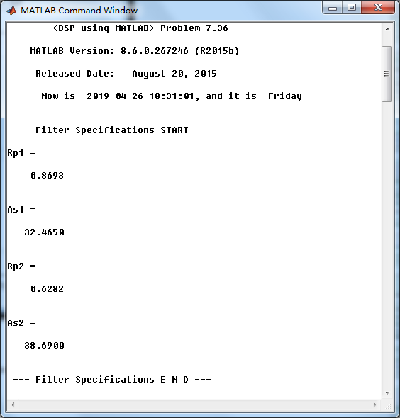
w1 = 0; w2 = 0.20*pi; delta1 = 0.05; gain1 = 0.00;
w3 = 0.25*pi; w4 = 0.45*pi; delta2 = 0.10; gain2 = 2.00;
w5 = 0.50*pi; w6 = 0.70*pi; delta3 = 0.05; gain3 = 0.00;
w7 = 0.75*pi; w8 = pi; delta4 = 0.15; gain4 = 4.15;
fprintf('
--- Filter Specifications START ---
');
Rp1 = -20*log10((gain2-delta2)/(gain2+delta2))
As1 = -20*log10(delta1/(gain2+delta2))
Rp2 = -20*log10((gain4-delta4)/(gain4+delta4))
As2 = -20*log10(delta3/(gain4+delta4))
fprintf('
--- Filter Specifications E N D ---
');
As = min(As1, As2);
fprintf('
--- Fix Window Method ---
');
tr_width = min((w3-w2), (w5-w4));
%% ---------------------------------------------------
%% 1 Rectangular Window
%% ---------------------------------------------------
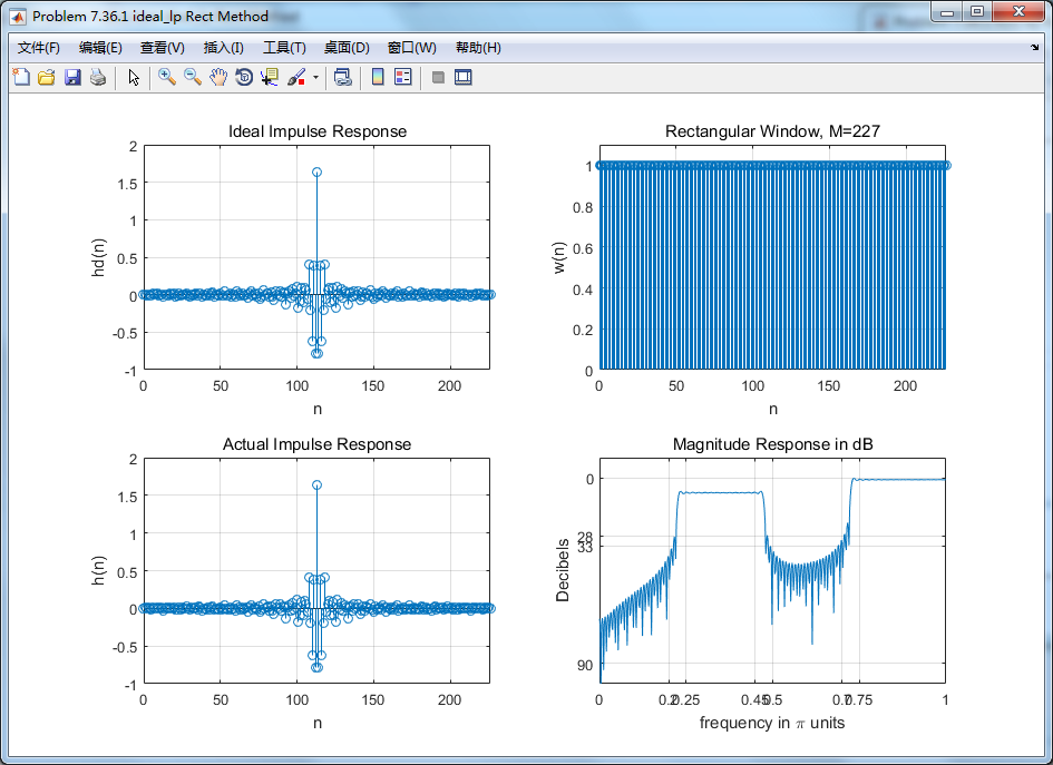
M = ceil(1.8*pi/tr_width) + 1; % Rectangular Window M=37
M=M+190;
fprintf('
#1.Rectangular Window, Filter Length M=%d.
', M);
n = [0:1:M-1]; wc1 = (w2+w3)/2; wc2 = (w4+w5)/2; wc3 = (w6+w7)/2;
hd = 2*(ideal_lp(wc2, M) - ideal_lp(wc1, M)) + 4.15*(ideal_lp(pi, M) - ideal_lp(wc3, M));
w_rect = (boxcar(M))'; h = hd .* w_rect;
[db, mag, pha, grd, w] = freqz_m(h, [1]); delta_w = 2*pi/1000;
[Hr,ww,P,L] = ampl_res(h);
w1i = floor(w1/delta_w)+1; w2i = floor(w2/delta_w)+1;
w3i = floor(w3/delta_w)+1; w4i = floor(w4/delta_w)+1;
w5i = floor(w5/delta_w)+1; w6i = floor(w6/delta_w)+1;
w7i = floor(w7/delta_w)+1; w8i = floor(w8/delta_w)+1;
Rp1 = -(min(db(w3i :1: w4i))); % Actual Passband Ripple
Rp2 = -(min(db(w7i :1: w8i))); % Actual Passband Ripple
fprintf('
Actual Passband Ripple is %.4f and %.4f dB.
', Rp1, Rp2);
As1 = -round(max(db(1 : 1 : w2i))); % Min Stopband attenuation
As2 = -round(max(db(w5i : 1 : w6i))); % Min Stopband attenuation
fprintf('
Min Stopband attenuation is %.4f and %.4f dB.
', As1, As2);
[delta1_rect1, delta2_rect1] = db2delta(Rp1, As1)
[delta1_rect2, delta2_rect2] = db2delta(Rp2, As2)
%% ----------------------------
%% Plot
%% -----------------------------
figure('NumberTitle', 'off', 'Name', 'Problem 7.36.1 ideal_lp Rect Method')
set(gcf,'Color','white');
subplot(2,2,1); stem(n, hd); axis([0 M-1 -1.0 2.0]); grid on;
xlabel('n'); ylabel('hd(n)'); title('Ideal Impulse Response');
subplot(2,2,2); stem(n, w_rect); axis([0 M-1 0 1.1]); grid on;
xlabel('n'); ylabel('w(n)'); title('Rectangular Window, M=227');
subplot(2,2,3); stem(n, h); axis([0 M-1 -1.0 2.0]); grid on;
xlabel('n'); ylabel('h(n)'); title('Actual Impulse Response');
subplot(2,2,4); plot(w/pi, db); axis([0 1 -100 10]); grid on;
set(gca,'YTickMode','manual','YTick',[-90,-33,-28,0]);
set(gca,'YTickLabelMode','manual','YTickLabel',['90';'33';'28';' 0']);
set(gca,'XTickMode','manual','XTick',[0,0.2,0.25,0.45,0.5,0.7,0.75,1]);
xlabel('frequency in pi units'); ylabel('Decibels'); title('Magnitude Response in dB');
figure('NumberTitle', 'off', 'Name', 'Problem 7.36.1 h(n) ideal_lp Rect Method')
set(gcf,'Color','white');
subplot(2,2,1); plot(w/pi, db); grid on; %axis([0 1 -100 10]);
xlabel('frequency in pi units'); ylabel('Decibels'); title('Magnitude Response in dB');
set(gca,'YTickMode','manual','YTick',[-90,-33,-28,0])
set(gca,'YTickLabelMode','manual','YTickLabel',['90';'33';'28';' 0']);
set(gca,'XTickMode','manual','XTick',[0,0.2,0.25,0.45,0.5,0.7,0.75,1,2]);
subplot(2,2,3); plot(w/pi, mag); grid on; %axis([0 1 -100 10]);
xlabel('frequency in pi units'); ylabel('Absolute'); title('Magnitude Response in absolute');
set(gca,'XTickMode','manual','XTick',[0,0.2,0.25,0.45,0.5,0.7,0.75,1,2]);
set(gca,'YTickMode','manual','YTick',[0.0,2.0,4.15])
subplot(2,2,2); plot(w/pi, pha); grid on; %axis([0 1 -100 10]);
xlabel('frequency in pi units'); ylabel('Rad'); title('Phase Response in Radians');
subplot(2,2,4); plot(w/pi, grd*pi/180); grid on; %axis([0 1 -100 10]);
xlabel('frequency in pi units'); ylabel('Rad'); title('Group Delay');
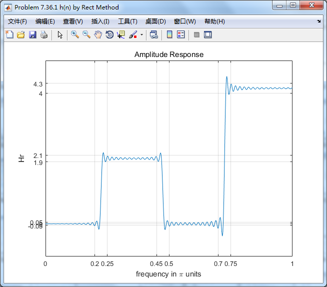
figure('NumberTitle', 'off', 'Name', 'Problem 7.36.1 h(n) by Rect Method')
set(gcf,'Color','white');
plot(ww/pi, Hr); grid on; %axis([0 1 -100 10]);
xlabel('frequency in pi units'); ylabel('Hr'); title('Amplitude Response');
set(gca,'YTickMode','manual','YTick',[-delta1, 0, delta1, 2-delta2, 2+ delta2, 4.15- delta4, 4.15+delta4])
set(gca,'XTickMode','manual','XTick',[0,0.2,0.25,0.45,0.5,0.7,0.75,1]);
%% ---------------------------------------------------
%% 2 Bartlett Window
%% ---------------------------------------------------
M = ceil(6.1*pi/tr_width) + 1; % Bartlett Window M=123
M=M+90;
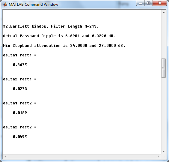
fprintf('
#2.Bartlett Window, Filter Length M=%d.
', M);
n = [0:1:M-1]; wc1 = (w2+w3)/2; wc2 = (w4+w5)/2; wc3 = (w6+w7)/2;
%wc = (ws + wp)/2, % ideal LPF cutoff frequency
hd = 2*(ideal_lp(wc2, M) - ideal_lp(wc1, M)) + 4.15*(ideal_lp(pi, M) - ideal_lp(wc3, M));
w_bart = (bartlett(M))'; h = hd .* w_bart;
[db, mag, pha, grd, w] = freqz_m(h, [1]); delta_w = 2*pi/1000;
[Hr,ww,P,L] = ampl_res(h);
Rp1 = -(min(db(w3i :1: w4i))); % Actual Passband Ripple
Rp2 = -(min(db(w7i :1: w8i))); % Actual Passband Ripple
fprintf('
Actual Passband Ripple is %.4f and %.4f dB.
', Rp1, Rp2);
As1 = -round(max(db(1 : 1 : w2i))); % Min Stopband attenuation
As2 = -round(max(db(w5i : 1 : w6i))); % Min Stopband attenuation
fprintf('
Min Stopband attenuation is %.4f and %.4f dB.
', As1, As2);
[delta1_rect1, delta2_rect1] = db2delta(Rp1, As1)
[delta1_rect2, delta2_rect2] = db2delta(Rp2, As2)
%% --------------------------
%% Plot
%% --------------------------
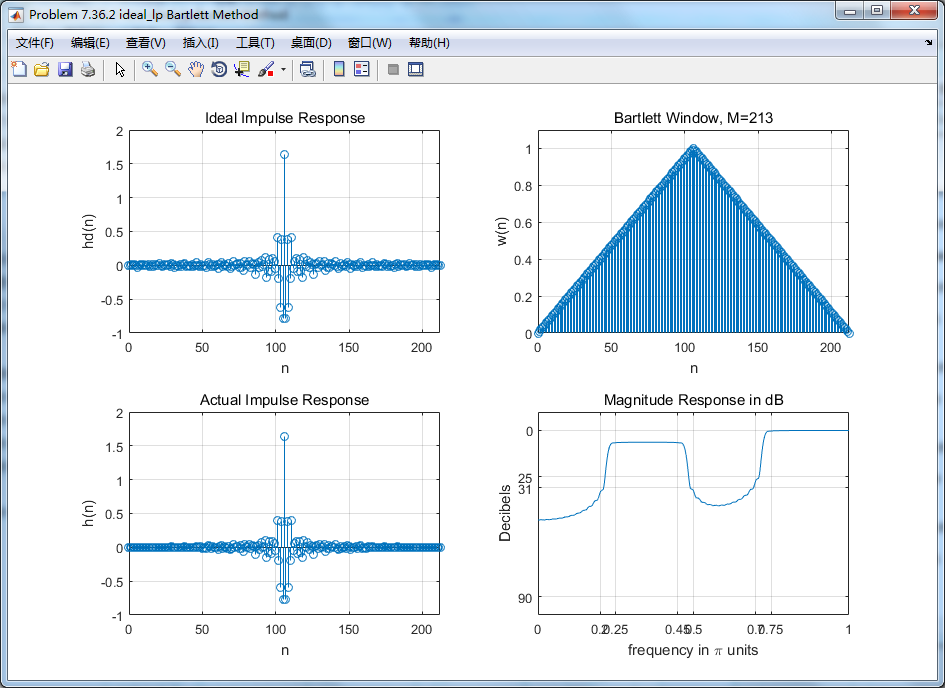
figure('NumberTitle', 'off', 'Name', 'Problem 7.36.2 ideal_lp Bartlett Method')
set(gcf,'Color','white');
subplot(2,2,1); stem(n, hd); axis([0 M-1 -1.0 2.0]); grid on;
xlabel('n'); ylabel('hd(n)'); title('Ideal Impulse Response');
subplot(2,2,2); stem(n, w_bart); axis([0 M-1 0 1.1]); grid on;
xlabel('n'); ylabel('w(n)'); title('Bartlett Window, M=213');
subplot(2,2,3); stem(n, h); axis([0 M-1 -1.0 2.0]); grid on;
xlabel('n'); ylabel('h(n)'); title('Actual Impulse Response');
subplot(2,2,4); plot(w/pi, db); axis([0 1 -100 10]); grid on;
set(gca,'YTickMode','manual','YTick',[-90,-31,-25,0]);
set(gca,'YTickLabelMode','manual','YTickLabel',['90';'31';'25';' 0']);
set(gca,'XTickMode','manual','XTick',[0,0.2,0.25,0.45,0.5,0.7,0.75,1]);
xlabel('frequency in pi units'); ylabel('Decibels'); title('Magnitude Response in dB');
figure('NumberTitle', 'off', 'Name', 'Problem 7.36.2 h(n) ideal_lp Bartlett Method')
set(gcf,'Color','white');
subplot(2,2,1); plot(w/pi, db); grid on; axis([0 2 -100 10]);
xlabel('frequency in pi units'); ylabel('Decibels'); title('Magnitude Response in dB');
set(gca,'YTickMode','manual','YTick',[-90,-31,-25,0])
set(gca,'YTickLabelMode','manual','YTickLabel',['90';'31';'25';' 0']);
set(gca,'XTickMode','manual','XTick',[0,0.2,0.25,0.45,0.5,0.7,0.75,1,2]);
subplot(2,2,3); plot(w/pi, mag); grid on; %axis([0 2 -100 10]);
xlabel('frequency in pi units'); ylabel('Absolute'); title('Magnitude Response in absolute');
set(gca,'XTickMode','manual','XTick',[0,0.2,0.25,0.45,0.5,0.7,0.75,1,2]);
set(gca,'YTickMode','manual','YTick',[0.0,2.0,4.15])
subplot(2,2,2); plot(w/pi, pha); grid on; %axis([0 1 -100 10]);
xlabel('frequency in pi units'); ylabel('Rad'); title('Phase Response in Radians');
subplot(2,2,4); plot(w/pi, grd*pi/180); grid on; %axis([0 1 -100 10]);
xlabel('frequency in pi units'); ylabel('Rad'); title('Group Delay');
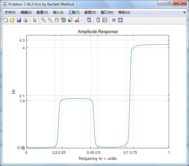
figure('NumberTitle', 'off', 'Name', 'Problem 7.36.2 h(n) by Bartlett Method')
set(gcf,'Color','white');
plot(ww/pi, Hr); grid on; %axis([0 1 -100 10]);
xlabel('frequency in pi units'); ylabel('Hr'); title('Amplitude Response');
set(gca,'YTickMode','manual','YTick',[-delta1, 0, delta1, 2-delta2, 2+ delta2, 4.15- delta4, 4.15+delta4])
set(gca,'XTickMode','manual','XTick',[0,0.2,0.25,0.45,0.5,0.7,0.75,1]);
%% ---------------------------------------------------
%% 3 Hann Window
%% ---------------------------------------------------
M = ceil(6.2*pi/tr_width) + 1; % Hann Window
fprintf('
#3.Hann Window, Filter Length M=%4d.
', M);
n = [0:1:M-1]; wc1 = (w2+w3)/2; wc2 = (w4+w5)/2; wc3 = (w6+w7)/2;
%wc = (ws + wp)/2, % ideal LPF cutoff frequency
hd = 2*(ideal_lp(wc2, M) - ideal_lp(wc1, M)) + 4.15*(ideal_lp(pi, M) - ideal_lp(wc3, M));
w_hann = (hann(M))'; h = hd .* w_hann;
[db, mag, pha, grd, w] = freqz_m(h, [1]); delta_w = 2*pi/1000;
[Hr,ww,P,L] = ampl_res(h);
Rp1 = -(min(db(w3i :1: w4i))); % Actual Passband Ripple
Rp2 = -(min(db(w7i :1: w8i))); % Actual Passband Ripple
fprintf('
Actual Passband Ripple is %.4f and %.4f dB.
', Rp1, Rp2);
As1 = -round(max(db(1 : 1 : w2i))); % Min Stopband attenuation
As2 = -round(max(db(w5i : 1 : w6i))); % Min Stopband attenuation
fprintf('
Min Stopband attenuation is %.4f and %.4f dB.
', As1, As2);
[delta1_rect1, delta2_rect1] = db2delta(Rp1, As1)
[delta1_rect2, delta2_rect2] = db2delta(Rp2, As2)
%% --------------------------
%% Plot
%% --------------------------
figure('NumberTitle', 'off', 'Name', 'Problem 7.36.3 ideal_lp Hann Method')
set(gcf,'Color','white');
subplot(2,2,1); stem(n, hd); axis([0 M-1 -1.0 2.0]); grid on;
xlabel('n'); ylabel('hd(n)'); title('Ideal Impulse Response');
subplot(2,2,2); stem(n, w_hann); axis([0 M-1 0 1.1]); grid on;
xlabel('n'); ylabel('w(n)'); title('Hann Window, M=125');
subplot(2,2,3); stem(n, h); axis([0 M-1 -1.0 2.0]); grid on;
xlabel('n'); ylabel('h(n)'); title('Actual Impulse Response');
subplot(2,2,4); plot(w/pi, db); axis([0 1 -100 10]); grid on;
set(gca,'YTickMode','manual','YTick',[-90,-49,-41,0]);
set(gca,'YTickLabelMode','manual','YTickLabel',['90';'49';'41';' 0']);
set(gca,'XTickMode','manual','XTick',[0,0.2,0.25,0.45,0.5,0.7,0.75,1]);
xlabel('frequency in pi units'); ylabel('Decibels'); title('Magnitude Response in dB');
figure('NumberTitle', 'off', 'Name', 'Problem 7.36.3 h(n) ideal_lp Hann Method')
set(gcf,'Color','white');
subplot(2,2,1); plot(w/pi, db); grid on; axis([0 2 -100 10]);
xlabel('frequency in pi units'); ylabel('Decibels'); title('Magnitude Response in dB');
set(gca,'YTickMode','manual','YTick',[-90,-49,-41,0])
set(gca,'YTickLabelMode','manual','YTickLabel',['90';'49';'41';' 0']);
set(gca,'XTickMode','manual','XTick',[0,0.2,0.25,0.45,0.5,0.7,0.75,1,2]);
subplot(2,2,3); plot(w/pi, mag); grid on; %axis([0 2 -100 10]);
xlabel('frequency in pi units'); ylabel('Absolute'); title('Magnitude Response in absolute');
set(gca,'XTickMode','manual','XTick',[0,0.2,0.25,0.45,0.5,0.7,0.75,1,2]);
set(gca,'YTickMode','manual','YTick',[0.0,2.0,4.15])
subplot(2,2,2); plot(w/pi, pha); grid on; %axis([0 1 -100 10]);
xlabel('frequency in pi units'); ylabel('Rad'); title('Phase Response in Radians');
subplot(2,2,4); plot(w/pi, grd*pi/180); grid on; %axis([0 1 -100 10]);
xlabel('frequency in pi units'); ylabel('Rad'); title('Group Delay');
figure('NumberTitle', 'off', 'Name', 'Problem 7.36.3 h(n) by Hann Method')
set(gcf,'Color','white');
plot(ww/pi, Hr); grid on; %axis([0 1 -100 10]);
xlabel('frequency in pi units'); ylabel('Hr'); title('Amplitude Response');
set(gca,'YTickMode','manual','YTick',[-delta1, 0, delta1, 2-delta2, 2+ delta2, 4.15- delta4, 4.15+delta4])
set(gca,'XTickMode','manual','XTick',[0,0.2,0.25,0.45,0.5,0.7,0.75,1]);
%% ---------------------------------------------------
%% 4 Hamming Window
%% ---------------------------------------------------
M = ceil(6.6*pi/tr_width) + 1; % Hamming Window
fprintf('
#4.Hamming Window, Filter Length M=%4d.
', M);
n = [0:1:M-1]; wc1 = (w2+w3)/2; wc2 = (w4+w5)/2; wc3 = (w6+w7)/2;
%wc = (ws + wp)/2, % ideal LPF cutoff frequency
hd = 2*(ideal_lp(wc2, M) - ideal_lp(wc1, M)) + 4.15*(ideal_lp(pi, M) - ideal_lp(wc3, M));
w_hamm = (hamming(M))'; h = hd .* w_hamm;
[db, mag, pha, grd, w] = freqz_m(h, [1]); delta_w = 2*pi/1000;
[Hr,ww,P,L] = ampl_res(h);
Rp1 = -(min(db(w3i :1: w4i))); % Actual Passband Ripple
Rp2 = -(min(db(w7i :1: w8i))); % Actual Passband Ripple
fprintf('
Actual Passband Ripple is %.4f and %.4f dB.
', Rp1, Rp2);
As1 = -round(max(db(1 : 1 : w2i))); % Min Stopband attenuation
As2 = -round(max(db(w5i : 1 : w6i))); % Min Stopband attenuation
fprintf('
Min Stopband attenuation is %.4f and %.4f dB.
', As1, As2);
[delta1_rect1, delta2_rect1] = db2delta(Rp1, As1)
[delta1_rect2, delta2_rect2] = db2delta(Rp2, As2)
%% --------------------------
%% Plot
%% --------------------------
figure('NumberTitle', 'off', 'Name', 'Problem 7.36.4 ideal_lp Hamming Method')
set(gcf,'Color','white');
subplot(2,2,1); stem(n, hd); axis([0 M-1 -1.0 2.0]); grid on;
xlabel('n'); ylabel('hd(n)'); title('Ideal Impulse Response');
subplot(2,2,2); stem(n, w_hamm); axis([0 M-1 0 1.1]); grid on;
xlabel('n'); ylabel('w(n)'); title('Hamming Window, M=133');
subplot(2,2,3); stem(n, h); axis([0 M-1 -1.0 2.0]); grid on;
xlabel('n'); ylabel('h(n)'); title('Actual Impulse Response');
subplot(2,2,4); plot(w/pi, db); axis([0 1 -100 10]); grid on;
set(gca,'YTickMode','manual','YTick',[-90,-59,-49,0]);
set(gca,'YTickLabelMode','manual','YTickLabel',['90';'59';'49';' 0']);
set(gca,'XTickMode','manual','XTick',[0,0.2,0.25,0.45,0.5,0.7,0.75,1]);
xlabel('frequency in pi units'); ylabel('Decibels'); title('Magnitude Response in dB');
figure('NumberTitle', 'off', 'Name', 'Problem 7.36.4 h(n) ideal_lp Hamming Method')
set(gcf,'Color','white');
subplot(2,2,1); plot(w/pi, db); grid on; axis([0 2 -100 10]);
xlabel('frequency in pi units'); ylabel('Decibels'); title('Magnitude Response in dB');
set(gca,'YTickMode','manual','YTick',[-90,-59,-49,0])
set(gca,'YTickLabelMode','manual','YTickLabel',['90';'59';'49';' 0']);
set(gca,'XTickMode','manual','XTick',[0,0.2,0.25,0.45,0.5,0.7,0.75,1,1.3,1.5,1.8,2]);
subplot(2,2,3); plot(w/pi, mag); grid on; %axis([0 2 -100 10]);
xlabel('frequency in pi units'); ylabel('Absolute'); title('Magnitude Response in absolute');
set(gca,'XTickMode','manual','XTick',[0,0.2,0.25,0.45,0.5,0.7,0.75,1,1.3,1.5,1.8,2]);
set(gca,'YTickMode','manual','YTick',[0.0,2.0,4.15])
subplot(2,2,2); plot(w/pi, pha); grid on; %axis([0 1 -100 10]);
xlabel('frequency in pi units'); ylabel('Rad'); title('Phase Response in Radians');
subplot(2,2,4); plot(w/pi, grd*pi/180); grid on; %axis([0 1 -100 10]);
xlabel('frequency in pi units'); ylabel('Rad'); title('Group Delay');
figure('NumberTitle', 'off', 'Name', 'Problem 7.36.4 h(n) by Hamming Method')
set(gcf,'Color','white');
plot(ww/pi, Hr); grid on; %axis([0 1 -100 10]);
xlabel('frequency in pi units'); ylabel('Hr'); title('Amplitude Response');
set(gca,'YTickMode','manual','YTick',[-delta1, 0, delta1, 2-delta2, 2+ delta2, 4.15- delta4, 4.15+delta4])
set(gca,'XTickMode','manual','XTick',[0,0.2,0.25,0.45,0.5,0.7,0.75,1]);
%% ---------------------------------------------------
%% 5 Blackman Window
%% ---------------------------------------------------
M = ceil(11*pi/tr_width) + 1; % Blackman Window
fprintf('
#5.Blackman Window, Filter Length M=%d.
', M);
n = [0:1:M-1]; wc1 = (w2+w3)/2; wc2 = (w4+w5)/2; wc3 = (w6+w7)/2;
%wc = (ws + wp)/2, % ideal LPF cutoff frequency
hd = 2*(ideal_lp(wc2, M) - ideal_lp(wc1, M)) + 4.15*(ideal_lp(pi, M) - ideal_lp(wc3, M));
w_bla = (blackman(M))'; h = hd .* w_bla;
[db, mag, pha, grd, w] = freqz_m(h, [1]); delta_w = 2*pi/1000;
[Hr,ww,P,L] = ampl_res(h);
Rp1 = -(min(db(w3i :1: w4i))); % Actual Passband Ripple
Rp2 = -(min(db(w7i :1: w8i))); % Actual Passband Ripple
fprintf('
Actual Passband Ripple is %.4f and %.4f dB.
', Rp1, Rp2);
As1 = -round(max(db(1 : 1 : w2i))); % Min Stopband attenuation
As2 = -round(max(db(w5i : 1 : w6i))); % Min Stopband attenuation
fprintf('
Min Stopband attenuation is %.4f and %.4f dB.
', As1, As2);
[delta1_rect1, delta2_rect1] = db2delta(Rp1, As1)
[delta1_rect2, delta2_rect2] = db2delta(Rp2, As2)
%% --------------------------
%% Plot
%% --------------------------
figure('NumberTitle', 'off', 'Name', 'Problem 7.36.5 ideal_lp Blackman Method')
set(gcf,'Color','white');
subplot(2,2,1); stem(n, hd); axis([0 M-1 -1.0 2.0]); grid on;
xlabel('n'); ylabel('hd(n)'); title('Ideal Impulse Response');
subplot(2,2,2); stem(n, w_bla); axis([0 M-1 0 1.1]); grid on;
xlabel('n'); ylabel('w(n)'); title('Blackman Window, M=221');
subplot(2,2,3); stem(n, h); axis([0 M-1 -1.0 2.0]); grid on;
xlabel('n'); ylabel('h(n)'); title('Actual Impulse Response');
subplot(2,2,4); plot(w/pi, db); axis([0 1 -120 10]); grid on;
set(gca,'YTickMode','manual','YTick',[-90,-80,-68,0]);
set(gca,'YTickLabelMode','manual','YTickLabel',['90';'80';'68';' 0']);
set(gca,'XTickMode','manual','XTick',[0,0.2,0.25,0.45,0.5,0.7,0.75,1]);
xlabel('frequency in pi units'); ylabel('Decibels'); title('Magnitude Response in dB');
figure('NumberTitle', 'off', 'Name', 'Problem 7.36.5 h(n) ideal_lp Blackman Method')
set(gcf,'Color','white');
subplot(2,2,1); plot(w/pi, db); grid on; axis([0 2 -120 10]);
xlabel('frequency in pi units'); ylabel('Decibels'); title('Magnitude Response in dB');
set(gca,'YTickMode','manual','YTick',[-90,-80,-68,0])
set(gca,'YTickLabelMode','manual','YTickLabel',['90';'80';'68';' 0']);
set(gca,'XTickMode','manual','XTick',[0,0.2,0.25,0.45,0.5,0.7,0.75,1,1.3,1.5,1.8,2]);
subplot(2,2,3); plot(w/pi, mag); grid on; %axis([0 2 -120 10]);
xlabel('frequency in pi units'); ylabel('Absolute'); title('Magnitude Response in absolute');
set(gca,'XTickMode','manual','XTick',[0,0.2,0.25,0.45,0.5,0.7,0.75,1,1.3,1.5,1.8,2]);
set(gca,'YTickMode','manual','YTick',[0.0,2.0,4.15])
subplot(2,2,2); plot(w/pi, pha); grid on; %axis([0 1 -100 10]);
xlabel('frequency in pi units'); ylabel('Rad'); title('Phase Response in Radians');
subplot(2,2,4); plot(w/pi, grd*pi/180); grid on; %axis([0 1 -100 10]);
xlabel('frequency in pi units'); ylabel('Rad'); title('Group Delay');
figure('NumberTitle', 'off', 'Name', 'Problem 7.16.5 h(n) by Blackman Method')
set(gcf,'Color','white');
plot(ww/pi, Hr); grid on; %axis([0 1 -100 10]);
xlabel('frequency in pi units'); ylabel('Hr'); title('Amplitude Response');
set(gca,'YTickMode','manual','YTick',[-delta1, 0, delta1, 2-delta2, 2+ delta2, 4.15- delta4, 4.15+delta4])
set(gca,'XTickMode','manual','XTick',[0,0.2,0.25,0.45,0.5,0.7,0.75,1]);
%% ---------------------------------------------------
%% 6 Kaiser Window
%% ---------------------------------------------------
As = 40;
M = ceil((As-7.95)/(2.285*tr_width)) + 1; % Kaiser Window 26--even
if As > 21 || As < 50
beta = 0.5842*(As-21)^0.4 + 0.07886*(As-21);
else
beta = 0.1102*(As-8.7);
end
fprintf('
#6.Kaiser Window, Filter Length M=%d, beta=%.4f
', M,beta);
n = [0:1:M-1]; wc1 = (w2+w3)/2; wc2 = (w4+w5)/2; wc3 = (w6+w7)/2;
%wc = (ws + wp)/2, % ideal LPF cutoff frequency
hd = 2*(ideal_lp(wc2, M) - ideal_lp(wc1, M)) + 4.15*(ideal_lp(pi, M) - ideal_lp(wc3, M));
w_kai = (kaiser(M,beta))'; h = hd .* w_kai;
[db, mag, pha, grd, w] = freqz_m(h, [1]); delta_w = 2*pi/1000;
[Hr,ww,P,L] = ampl_res(h);
Rp1 = -(min(db(w3i :1: w4i))); % Actual Passband Ripple
Rp2 = -(min(db(w7i :1: w8i))); % Actual Passband Ripple
fprintf('
Actual Passband Ripple is %.4f and %.4f dB.
', Rp1, Rp2);
As1 = -round(max(db(1 : 1 : w2i))); % Min Stopband attenuation
As2 = -round(max(db(w5i : 1 : w6i))); % Min Stopband attenuation
fprintf('
Min Stopband attenuation is %.4f and %.4f dB.
', As1, As2);
[delta1_rect1, delta2_rect1] = db2delta(Rp1, As1)
[delta1_rect2, delta2_rect2] = db2delta(Rp2, As2)
%% --------------------------
%% Plot
%% --------------------------
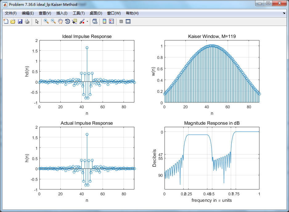
figure('NumberTitle', 'off', 'Name', 'Problem 7.36.6 ideal_lp Kaiser Method')
set(gcf,'Color','white');
subplot(2,2,1); stem(n, hd); axis([0 M-1 -1.0 2.0]); grid on;
xlabel('n'); ylabel('hd(n)'); title('Ideal Impulse Response');
subplot(2,2,2); stem(n, w_kai); axis([0 M-1 0 1.1]); grid on;
xlabel('n'); ylabel('w(n)'); title('Kaiser Window, M=119');
subplot(2,2,3); stem(n, h); axis([0 M-1 -1.0 2.0]); grid on;
xlabel('n'); ylabel('h(n)'); title('Actual Impulse Response');
subplot(2,2,4); plot(w/pi, db); axis([0 1 -120 10]); grid on;
set(gca,'YTickMode','manual','YTick',[-90,-55,-47,0]);
set(gca,'YTickLabelMode','manual','YTickLabel',['90';'55';'47';' 0']);
set(gca,'XTickMode','manual','XTick',[0,0.2,0.25,0.45,0.5,0.7,0.75,1]);
xlabel('frequency in pi units'); ylabel('Decibels'); title('Magnitude Response in dB');
figure('NumberTitle', 'off', 'Name', 'Problem 7.36.6 h(n) ideal_lp Kaiser Method')
set(gcf,'Color','white');
subplot(2,2,1); plot(w/pi, db); grid on; axis([0 2 -120 10]);
xlabel('frequency in pi units'); ylabel('Decibels'); title('Magnitude Response in dB');
set(gca,'YTickMode','manual','YTick',[-90,-55,-47,0])
set(gca,'YTickLabelMode','manual','YTickLabel',['90';'55';'47';' 0']);
set(gca,'XTickMode','manual','XTick',[0,0.2,0.25,0.45,0.5,0.7,0.75,1,1.3,1.5,1.8,2]);
subplot(2,2,3); plot(w/pi, mag); grid on; %axis([0 2 -100 10]);
xlabel('frequency in pi units'); ylabel('Absolute'); title('Magnitude Response in absolute');
set(gca,'XTickMode','manual','XTick',[0,0.2,0.25,0.45,0.5,0.7,0.75,1,1.3,1.5,1.8,2]);
set(gca,'YTickMode','manual','YTick',[0.0,2.0,4.15])
subplot(2,2,2); plot(w/pi, pha); grid on; %axis([0 1 -100 10]);
xlabel('frequency in pi units'); ylabel('Rad'); title('Phase Response in Radians');
subplot(2,2,4); plot(w/pi, grd*pi/180); grid on; %axis([0 1 -100 10]);
xlabel('frequency in pi units'); ylabel('Rad'); title('Group Delay');
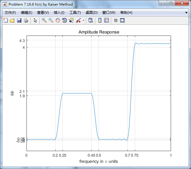
figure('NumberTitle', 'off', 'Name', 'Problem 7.16.6 h(n) by Kaiser Method')
set(gcf,'Color','white');
plot(ww/pi, Hr); grid on; %axis([0 1 -100 10]);
xlabel('frequency in pi units'); ylabel('Hr'); title('Amplitude Response');
set(gca,'YTickMode','manual','YTick',[-delta1, 0, delta1, 2-delta2, 2+ delta2, 4.15- delta4, 4.15+delta4])
set(gca,'XTickMode','manual','XTick',[0,0.2,0.25,0.45,0.5,0.7,0.75,1]);
运行结果:
窗函数法,使用了矩形窗、三角窗、Hann窗、Hamming窗、Blackman窗、Kaiser窗,
1、Rectangular窗

2、Bartlett三角窗
3、Hann、Hamming窗、Blackman窗的图这里不放了,直接放Kaiser窗的结果

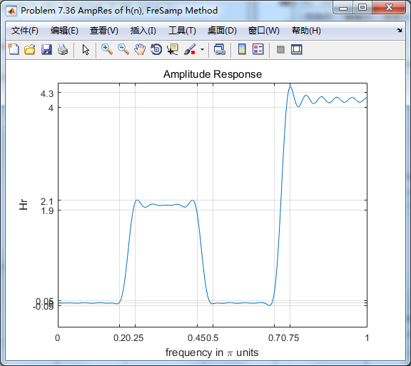
4、频率采样方法


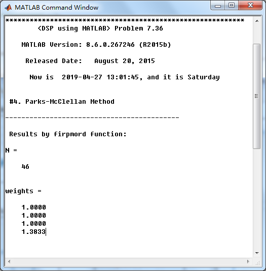
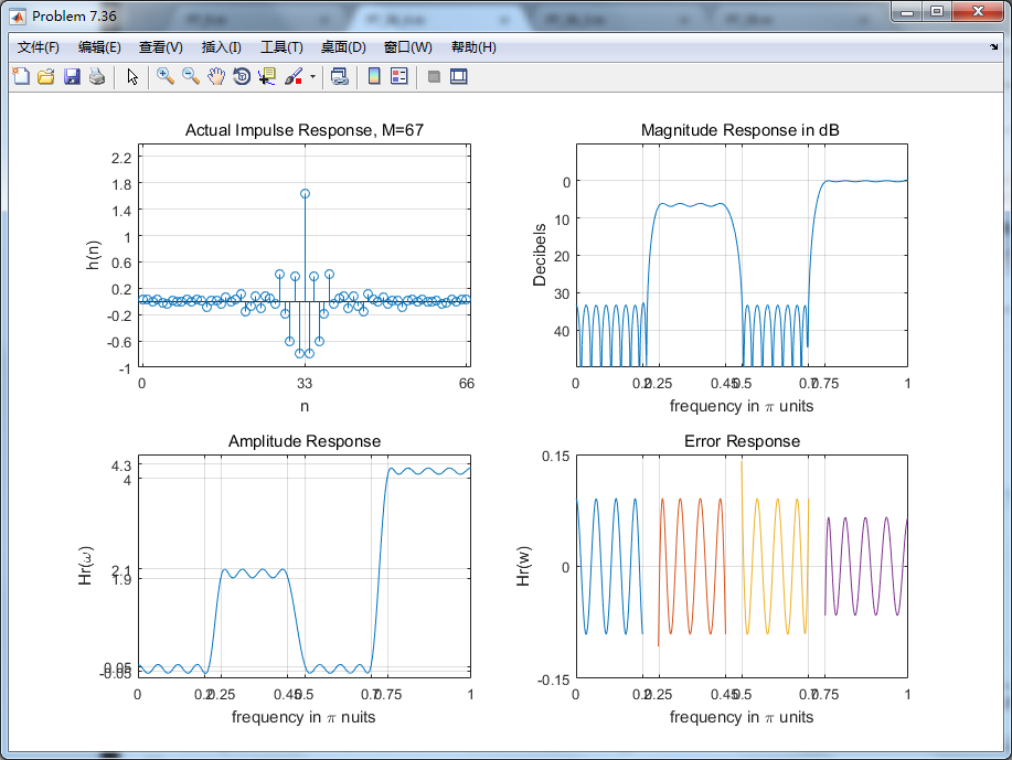
5、PM法

6、小结
以上用了窗函数法、频率采样法、Parks-McClellan法,下面对其得到的滤波器长度作对比,
| 序号 | 设 计 方 法 |
滤波器长度 M |
阻带衰减 As(dB) |
| 1 |
Rectangular矩形窗 |
227 | 28 |
| 2 | Bartlett三角窗 | 213 | 27 |
| 3 | Hann窗 | 125 | 41 |
| 4 | Hamming窗 | 133 | 49 |
| 5 | Blackman窗 | 221 | 68 |
| 6 | Kaiser窗 | 91 | 39 |
| 7 | 频率采样法 | 81 | 47 |
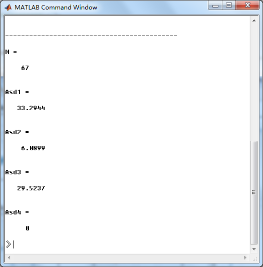
| 8 | Parks-McClellan法 | 67 | 30 |
结合滤波器指标要求和实际情况,Kaiser窗、频率采样法和P-M法可以采用。