又到清明时节,……


注意:带阻滤波器不能用第2类线性相位滤波器实现,我们采用第1类,长度为基数,选M=61
代码:
%% ++++++++++++++++++++++++++++++++++++++++++++++++++++++++++++++++++++++++++++++++
%% Output Info about this m-file
fprintf('
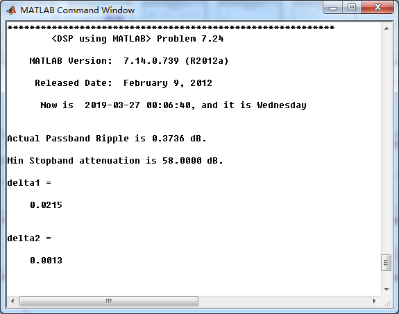
***********************************************************
');
fprintf(' <DSP using MATLAB> Problem 7.24
');
banner();
%% ++++++++++++++++++++++++++++++++++++++++++++++++++++++++++++++++++++++++++++++++
% bandstop filter
% Type-2 FIR ---- No highpass or bandstop
wp1 = 0.3*pi; ws1 = 0.4*pi; ws2 = 0.6*pi; wp2 = 0.7*pi;
As = 50; Rp = 0.2;
tr_width = min( ws1-wp1, wp2-ws2 );
T1 = 0.5925; T2=0.1099;
M = 61; alpha = (M-1)/2; l = 0:M-1; wl = (2*pi/M)*l;
n = [0:1:M-1]; wc1 = (ws1+wp1)/2; wc2 = (wp2+ws2)/2;
Hrs = [ones(1,10),T1,T2,zeros(1,7),T2,T1,ones(1,20),T1,T2,zeros(1,7),T2,T1,ones(1,9)]; % Ideal Amp Res sampled
Hdr = [1, 1, 0, 0, 1, 1]; wdl = [0, 0.3, 0.4, 0.6, 0.7, 1]; % Ideal Amp Res for plotting
k1 = 0:floor((M-1)/2); k2 = floor((M-1)/2)+1:M-1;
%% ----------------------------------
%% Type-1 LPF
%% ----------------------------------
angH = [-alpha*(2*pi)/M*k1, alpha*(2*pi)/M*(M-k2)];
H = Hrs.*exp(j*angH); h = real(ifft(H, M));
[db, mag, pha, grd, w] = freqz_m(h, 1); delta_w = 2*pi/1000;
[Hr, ww, a, L] = Hr_Type1(h);
Rp = -(min(db(1 :1: floor(wp1/delta_w)))); % Actual Passband Ripple
fprintf('
Actual Passband Ripple is %.4f dB.
', Rp);
As = -round(max(db(floor(ws1/delta_w)+1 : 1 : 0.55*pi/delta_w))); % Min Stopband attenuation
fprintf('
Min Stopband attenuation is %.4f dB.
', As);
[delta1, delta2] = db2delta(Rp, As)
%Plot
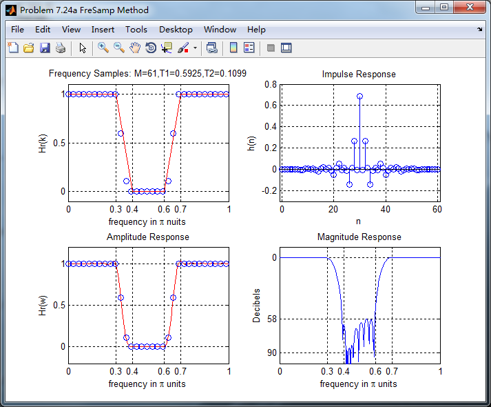
figure('NumberTitle', 'off', 'Name', 'Problem 7.24a FreSamp Method')
set(gcf,'Color','white');
subplot(2,2,1); plot(wl(1:31)/pi, Hrs(1:31), 'o', wdl, Hdr, 'r'); axis([0, 1, -0.1, 1.1]);
set(gca,'YTickMode','manual','YTick',[0,0.5,1]);
set(gca,'XTickMode','manual','XTick',[0,0.3,0.4,0.6,0.7,1]);
xlabel('frequency in pi nuits'); ylabel('Hr(k)'); title('Frequency Samples: M=61,T1=0.5925,T2=0.1099');
grid on;
subplot(2,2,2); stem(l, h); axis([-1, M, -0.3, 0.8]); grid on;
xlabel('n'); ylabel('h(n)'); title('Impulse Response');
subplot(2,2,3); plot(ww/pi, Hr, 'r', wl(1:31)/pi, Hrs(1:31), 'o'); axis([0, 1, -0.2, 1.2]); grid on;
xlabel('frequency in pi units'); ylabel('Hr(w)'); title('Amplitude Response');
set(gca,'YTickMode','manual','YTick',[0,0.5,1]);
set(gca,'XTickMode','manual','XTick',[0,0.3,0.4,0.6,0.7,1]);
subplot(2,2,4); plot(w/pi, db); axis([0, 1, -100, 10]); grid on;
xlabel('frequency in pi units'); ylabel('Decibels'); title('Magnitude Response');
set(gca,'YTickMode','manual','YTick',[-90,-58,0]);
set(gca,'YTickLabelMode','manual','YTickLabel',['90';'58';' 0']);
set(gca,'XTickMode','manual','XTick',[0,0.3,0.4,0.6,0.7,1]);
figure('NumberTitle', 'off', 'Name', 'Problem 7.24 h(n) FreSamp Method')
set(gcf,'Color','white');
subplot(2,2,1); plot(w/pi, db); grid on; axis([0 1 -120 10]);
set(gca,'YTickMode','manual','YTick',[-90,-58,0])
set(gca,'YTickLabelMode','manual','YTickLabel',['90';'58';' 0']);
set(gca,'XTickMode','manual','XTick',[0,0.3,0.4,0.6,0.7,1]);
xlabel('frequency in pi units'); ylabel('Decibels'); title('Magnitude Response in dB');
subplot(2,2,3); plot(w/pi, mag); grid on; %axis([0 1 -100 10]);
xlabel('frequency in pi units'); ylabel('Absolute'); title('Magnitude Response in absolute');
set(gca,'XTickMode','manual','XTick',[0,0.3,0.4,0.6,0.7,1,1.3,1.4,1.6,1.7,2]);
set(gca,'YTickMode','manual','YTick',[0,1.0]);
subplot(2,2,2); plot(w/pi, pha); grid on; %axis([0 1 -100 10]);
xlabel('frequency in pi units'); ylabel('Rad'); title('Phase Response in Radians');
subplot(2,2,4); plot(w/pi, grd*pi/180); grid on; %axis([0 1 -100 10]);
xlabel('frequency in pi units'); ylabel('Rad'); title('Group Delay');
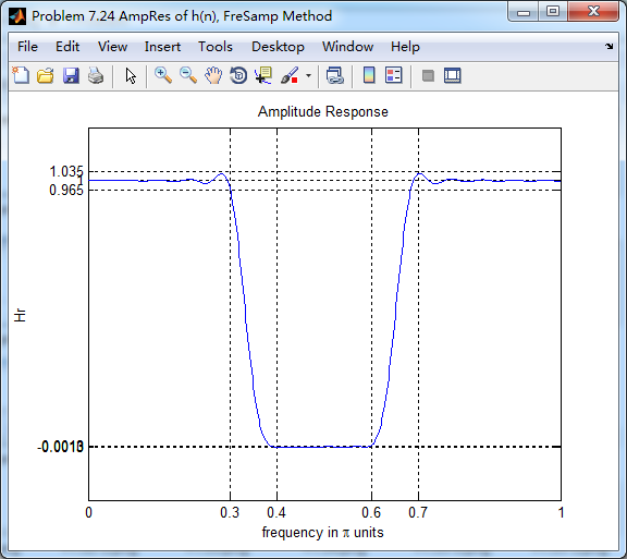
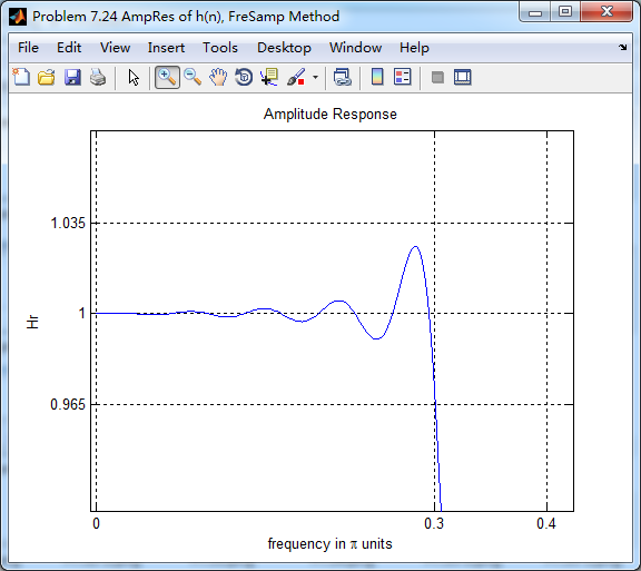
figure('NumberTitle', 'off', 'Name', 'Problem 7.24 AmpRes of h(n), FreSamp Method')
set(gcf,'Color','white');
plot(ww/pi, Hr); grid on; %axis([0 1 -100 10]);
xlabel('frequency in pi units'); ylabel('Hr'); title('Amplitude Response');
set(gca,'YTickMode','manual','YTick',[-delta2, 0,delta2, 1-0.035, 1,1+0.035]);
%set(gca,'YTickLabelMode','manual','YTickLabel',['90';'45';' 0']);
set(gca,'XTickMode','manual','XTick',[0,0.3,0.4,0.6,0.7,1]);
%% ------------------------------------
%% fir2 Method
%% ------------------------------------
f = [0 wp1 ws1 ws2 wp2 pi]/pi;
m = [1 1 0 0 1 1];
h_check = fir2(M+1, f, m); % if M is odd, then M+1; order
[db, mag, pha, grd, w] = freqz_m(h_check, [1]);
%[Hr,ww,P,L] = ampl_res(h_check);
[Hr, ww, a, L] = Hr_Type1(h_check);
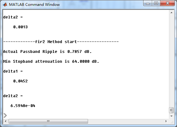
fprintf('
-------------fir2 Method start-----------------
');
Rp = -(min(db(1 :1: floor(wp1/delta_w)))); % Actual Passband Ripple
fprintf('
Actual Passband Ripple is %.4f dB.
', Rp);
%As = -round(max(db(floor(0.45*pi/delta_w)+1 : 1 : ws2/delta_w))); % Min Stopband attenuation
As = -round(max(db(floor(0.45*pi/delta_w)+1 : 1 : 0.55*pi/delta_w)));
fprintf('
Min Stopband attenuation is %.4f dB.
', As);
[delta1, delta2] = db2delta(Rp, As)
figure('NumberTitle', 'off', 'Name', 'Problem 7.24 fir2 Method')
set(gcf,'Color','white');
subplot(2,2,1); stem(n, h); axis([0 M-1 -0.3 0.8]); grid on;
xlabel('n'); ylabel('h(n)'); title('Impulse Response');
%subplot(2,2,2); stem(n, w_ham); axis([0 M-1 0 1.1]); grid on;
%xlabel('n'); ylabel('w(n)'); title('Hamming Window');
subplot(2,2,3); stem([0:M+1], h_check); axis([0 M+1 -0.3 0.8]); grid on;
xlabel('n'); ylabel('h\_check(n)'); title('Actual Impulse Response');
subplot(2,2,4); plot(w/pi, db); axis([0 1 -120 10]); grid on;
set(gca,'YTickMode','manual','YTick',[-90,-64,-21,0])
set(gca,'YTickLabelMode','manual','YTickLabel',['90';'64';'21';' 0']);
set(gca,'XTickMode','manual','XTick',[0,0.3,0.4,0.6,0.7,1]);
xlabel('frequency in pi units'); ylabel('Decibels'); title('Magnitude Response in dB');
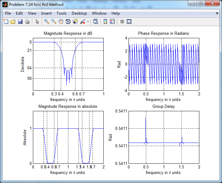
figure('NumberTitle', 'off', 'Name', 'Problem 7.24 h(n) fir2 Method')
set(gcf,'Color','white');
subplot(2,2,1); plot(w/pi, db); grid on; axis([0 1 -120 10]);
xlabel('frequency in pi units'); ylabel('Decibels'); title('Magnitude Response in dB');
set(gca,'YTickMode','manual','YTick',[-90,-64,-21,0]);
set(gca,'YTickLabelMode','manual','YTickLabel',['90';'64';'21';' 0']);
set(gca,'XTickMode','manual','XTick',[0,0.3,0.4,0.6,0.7,1,1.3,1.4,1.6,1.7,2]);
subplot(2,2,3); plot(w/pi, mag); grid on; %axis([0 1 -100 10]);
xlabel('frequency in pi units'); ylabel('Absolute'); title('Magnitude Response in absolute');
set(gca,'XTickMode','manual','XTick',[0,0.3,0.4,0.6,0.7,1,1.3,1.4,1.6,1.7,2]);
set(gca,'YTickMode','manual','YTick',[0,1.0]);
subplot(2,2,2); plot(w/pi, pha); grid on; %axis([0 1 -100 10]);
xlabel('frequency in pi units'); ylabel('Rad'); title('Phase Response in Radians');
subplot(2,2,4); plot(w/pi, grd*pi/180); grid on; %axis([0 1 -100 10]);
xlabel('frequency in pi units'); ylabel('Rad'); title('Group Delay');
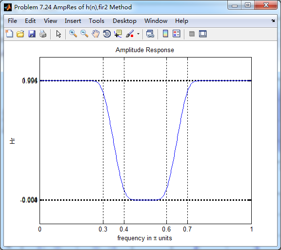
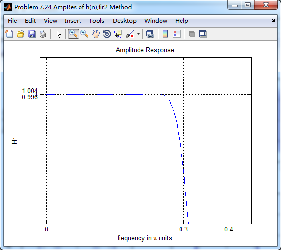
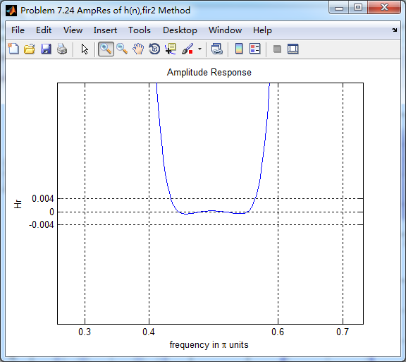
figure('NumberTitle', 'off', 'Name', 'Problem 7.24 AmpRes of h(n),fir2 Method')
set(gcf,'Color','white');
plot(ww/pi, Hr); grid on; %axis([0 1 -100 10]);
xlabel('frequency in pi units'); ylabel('Hr'); title('Amplitude Response');
set(gca,'YTickMode','manual','YTick',[-0.004, 0,0.004, 1-0.004, 1,1+0.004]);
%set(gca,'YTickLabelMode','manual','YTickLabel',['90';'45';' 0']);
set(gca,'XTickMode','manual','XTick',[0,0.3,0.4,0.6,0.7,1]);
运行结果:
过渡带中有两个采样值,优化值直接抄书上的。

采用频率采样方法得到的脉冲响应

采用fir2函数 的方法得到滤波器脉冲响应