单层感知机
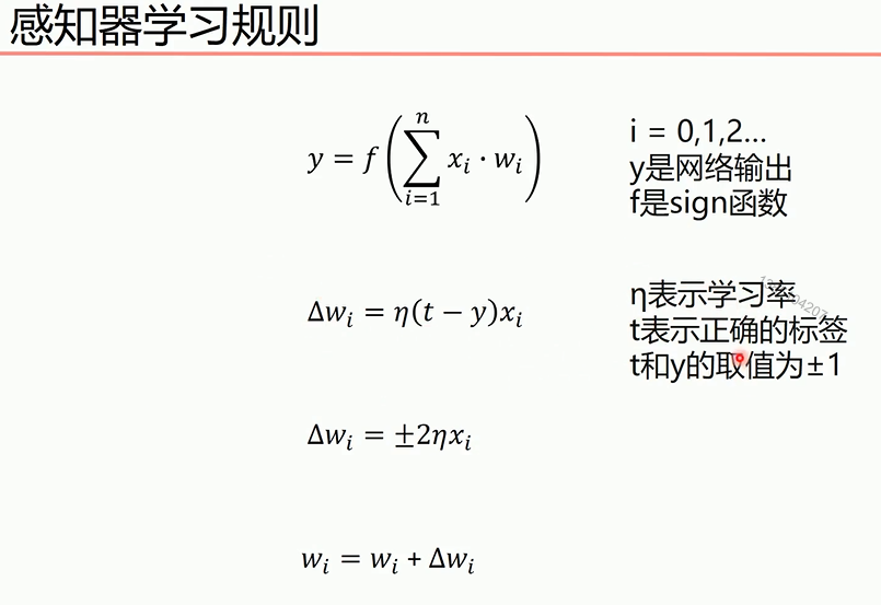
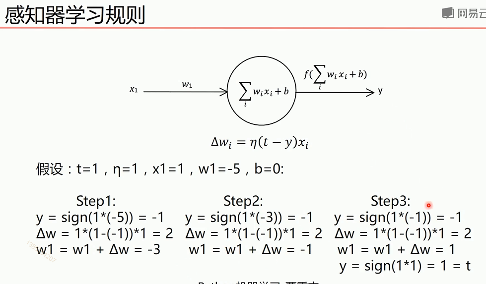
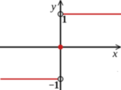
最终y=t,说明经过训练预测值和真实值一致。下面图是sign函数


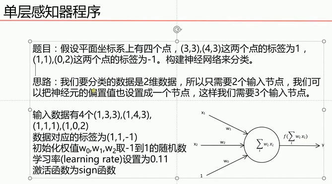
根据感知机规则实现的上述题目的代码
 1 import numpy as np
 2 import matplotlib.pyplot as plt
 3 #输入数据
 4 X = np.array([[1,3,3],
 5               [1,4,3],
 6               [1,1,1],
 7               [1,0,2]])
 8 #标签
 9 Y = np.array([[1],
10               [1],
11               [-1],
12               [-1]])
13 #权值初始化,3行1列,取值范围-1到1
14 W = (np.random.random([3,1])-0.5)*2
15 print(W)
16 #学习率设置
17 lr = 0.11
18 #神经网络输出
19 O = 0
20
21 def update():
22     global X,Y,W,lr
23     O = np.sign(np.dot(X,W))
24     W_C = lr*(X.T.dot(Y-O))/int(X.shape[0])#除于样本个数目的是分子计算的误差是所有样本误差之和,所以要进行平均
25     W = W + W_C
26 for i in range(100):
27     update()#更新权值
28     print(W)
29     print(i)
30     O = np.sign(np.dot(X,W))
31     if(O == Y).all():
32         print('finished')
33         print('epoch:',i)
34         break
35 #正样本
36 x1 = [3,4]
37 y1 = [3,3]
38     #负样本
39 x2 = [1,0]
40 y2 = [1,2]
41
42     #计算分界线的斜率以及截距
43 k = -W[1]/W[2]
44 d = -W[0]/W[2]
45 print('k=',k)
46 print('d=',d)
47
48 xdata = (0,5)
49
50 plt.figure()
51 plt.plot(xdata,xdata*k+d,'r')
52 plt.scatter(x1,y1,c='b')
53 plt.scatter(x2,y2,c='y')
54 plt.show()
单层感知机解决异或问题
 1 '''
 2 异或
 3 0^0 = 0
 4 0^1 = 1
 5 1^0 = 1
 6 1^1 = 0
 7 '''
 8 import numpy as np
 9 import matplotlib.pyplot as plt
10 #输入数据
11 X = np.array([[1,0,0],
12               [1,0,1],
13               [1,1,0],
14               [1,1,1]])
15 #标签
16 Y = np.array([[-1],
17               [1],
18               [1],
19               [-1]])
20
21 #权值初始化,3行1列,取值范围-1到1
22 W = (np.random.random([3,1])-0.5)*2
23
24 print(W)
25 #学习率设置
26 lr = 0.11
27 #神经网络输出
28 O = 0
29
30 def update():
31     global X,Y,W,lr
32     O = np.sign(np.dot(X,W)) # shape:(3,1)
33     W_C = lr*(X.T.dot(Y-O))/int(X.shape[0])
34     W = W + W_C
35 for i in range(100):
36     update()#更新权值
37     print(W)#打印当前权值
38     print(i)#打印迭代次数
39     O = np.sign(np.dot(X,W))#计算当前输出
40     if(O == Y).all(): #如果实际输出等于期望输出,模型收敛,循环结束
41         print('Finished')
42         print('epoch:',i)
43         break
44
45 #正样本
46 x1 = [0,1]
47 y1 = [1,0]
48 #负样本
49 x2 = [0,1]
50 y2 = [0,1]
51
52 #计算分界线的斜率以及截距
53 k = -W[1]/W[2]
54 d = -W[0]/W[2]
55 print('k=',k)
56 print('d=',d)
57
58 xdata = (-2,3)
59
60 plt.figure()
61 plt.plot(xdata,xdata*k+d,'r')
62 plt.scatter(x1,y1,c='b')
63 plt.scatter(x2,y2,c='y')
64 plt.show()
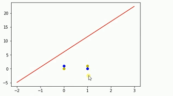
运行结果如上,可以知道单层感知机不适合解决如上类似的异或问题
线性神经网络
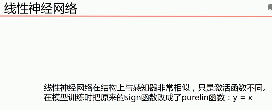
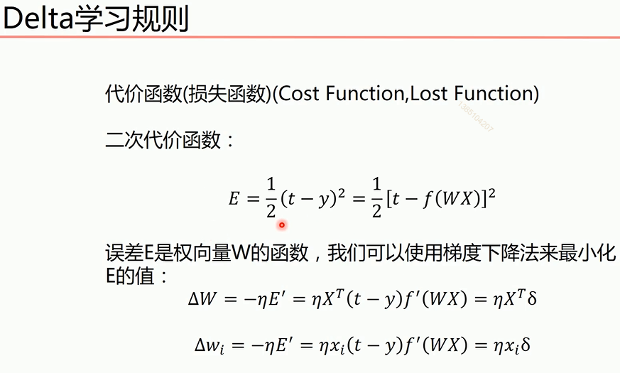
同时相比于感知机引入了Delta学习规则

解决感知机无法处理异或问题的方法
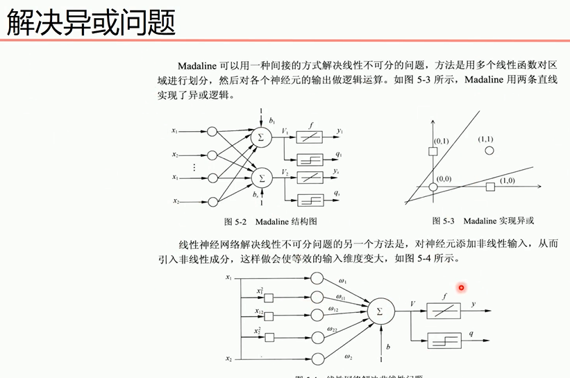
对于第二个方法

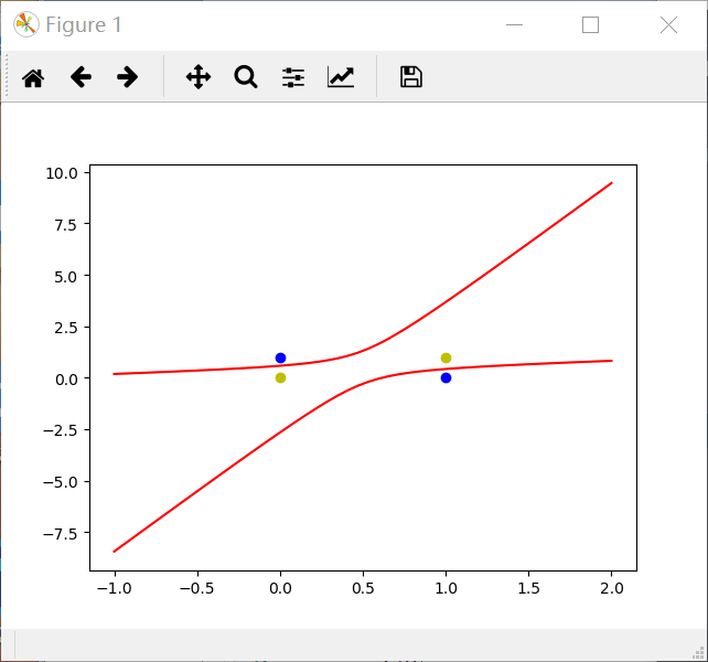
说明:X0是偏置值,值为1,X1,X2为线性输入,其它为添加的非线性输入,使用purelin激活函数(y=x)进行模型训练,再下面是y值的求法,用于图形绘制。
程序如下
 1 #题目:异或运算
 2 #0^0=0
 3 #0^1=1
 4 #1^0=1
 5 #1^1=0
 6 import numpy as np
 7 import matplotlib.pyplot as plt
 8 #输入数据--这里偏置定为1
 9 X = np.array([[1,0,0,0,0,0],
10               [1,0,1,0,0,1],
11               [1,1,0,1,0,0],
12               [1,1,1,1,1,1]])
13 #标签--期望输出
14 Y = np.array([-1,1,1,-1])
15 #权值初始化,1行6列,取-1到1的随机数
16 W = (np.random.random(6)-0.5)*2
17 print(W)
18 #学习率
19 lr = 0.11
20 #计算迭代次数
21 n = 0
22 #神经网络输出
23 o = 0
24
25 def update():
26     global X,Y,W,lr,n
27     n+=1
28     o = np.dot(X,W.T)
29     W_C = lr*((Y-o.T).dot(X))/(X.shape[0])#权值改变数,这里除掉行数求平均值,因为行数多,权值改变就会很大。
30     W = W + W_C
31 for  i in range(1000):
32     update()#更新权值
33
34 o = np.dot(X,W.T)
35 print("执行一千次后的输出结果:",o)#看下执行一千次之后的输出
36
37 #用图形表示出来
38 #正样本
39 x1 = [0,1]
40 y1 = [1,0]
41 #负样本
42 x2 = [0,1]
43 y2 = [0,1]
44
45 def calculate(x,root):
46     a = W[5]
47     b = W[2]+x*W[4]
48     c = W[0]+x*W[1]+x*x*W[3]
49     if root == 1:#第一个根
50         return (-b+np.sqrt(b*b-4*a*c))/(2*a)
51     if root == 2:#第二个根
52         return (-b-np.sqrt(b*b-4*a*c))/(2*a)
53
54 xdata = np.linspace(-1,2)
55
56 plt.figure()
57 plt.plot(xdata,calculate(xdata,1),'r')#用红色
58 plt.plot(xdata,calculate(xdata,2),'r')#用红色
59 plt.plot(x1,y1,'bo')#用蓝色
60 plt.plot(x2,y2,'yo')#用黄色
61 plt.show()
利用神经网络解决上述感知机题目
 1 import numpy as np
 2 import matplotlib.pyplot as plt
 3 #输入数据
 4 X = np.array([[1,3,3],
 5               [1,4,3],
 6               [1,1,1],
 7               [1,0,2]])
 8 #标签
 9 Y = np.array([[1],
10               [1],
11               [-1],
12               [-1]])
13
14 #权值初始化,3行1列,取值范围-1到1
15 W = (np.random.random([3,1])-0.5)*2
16
17 print(W)
18 #学习率设置
19 lr = 0.11
20 #神经网络输出
21 O = 0
22
23 def update():
24     global X,Y,W,lr
25     O = np.dot(X,W)
26     W_C = lr*(X.T.dot(Y-O))/int(X.shape[0])
27     W = W + W_C
28 for i in range(100):
29     update()#更新权值
30
31     #正样本
32     x1 = [3,4]
33     y1 = [3,3]
34     #负样本
35     x2 = [1,0]
36     y2 = [1,2]
37
38     #计算分界线的斜率以及截距
39     k = -W[1]/W[2]
40     d = -W[0]/W[2]
41     print('k=',k)
42     print('d=',d)
43
44     xdata = (0,5)
45     if i % 10 == 0:
46         plt.figure()
47         plt.plot(xdata,xdata*k+d,'r')
48         plt.scatter(x1,y1,c='b')
49         plt.scatter(x2,y2,c='y')
50         plt.show()
BP神经网络
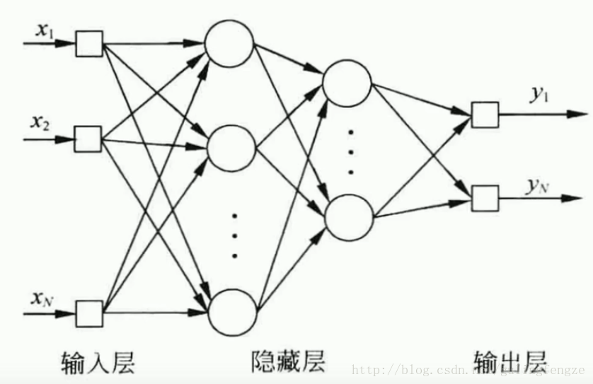
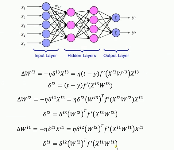
反向传播(Back Propagation,简称BP)神经网络解决了多层神经网络的学习问题,广泛应用于分类识别、图像识别、压缩、逼近以及回归等领域,其结构如下所示。
另外介绍及格激活函数:sigmoid、tanh和softsign。神经网络中的激活函数,其作用就是引入非线性。
Sigmoid:sigmoid的优点是输出范围有限,数据在传递的过程中不容易发散,求导很容易(y=sigmoid(x), y’=y(1-y))。缺点是饱和的时候梯度太小。其输出范围为(0, 1),所以可以用作输出层,输出表示概率。

公式:
Sigmoid:sigmoid的优点是输出范围有限,数据在传递的过程中不容易发散,求导很容易(y=sigmoid(x), y’=y(1-y))。缺点是饱和的时候梯度太小。其输出范围为(0, 1),所以可以用作输出层,输出表示概率。
公式:
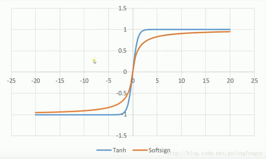
tanh和softsign:
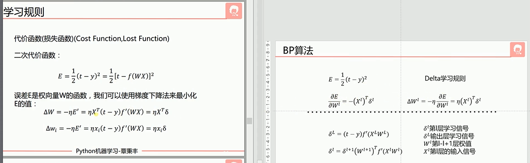
要注意的是对多层神经元先对最后一层权重更新,其结果再更新前一层的权重
bp神经网络解决异或问题的程序如下
 1 import numpy as np
 2
 3 # 输入数据
 4 X = np.array([[1, 0, 0],
 5               [1, 0, 1],
 6               [1, 1, 0],
 7               [1, 1, 1]])
 8 # 标签
 9 Y = np.array([[0, 1, 1, 0]])
10 # 权值初始化,取值范围-1到1
11 V = np.random.random((3, 4)) * 2 - 1
12 W = np.random.random((4, 1)) * 2 - 1
13 print(V)
14 print(W)
15 # 学习率设置
16 lr = 0.11
17 def sigmoid(x):
18     return 1 / (1 + np.exp(-x))
19 def dsigmoid(x):
20     return x * (1 - x)#激活函数的导数
21 def update():
22     global X, Y, W, V, lr
23
24     L1 = sigmoid(np.dot(X, V))  # 隐藏层输出(4,4)
25     L2 = sigmoid(np.dot(L1, W))  # 输出层输出(4,1)
26
27     L2_delta = (Y.T - L2) * dsigmoid(L2)
28     L1_delta = L2_delta.dot(W.T) * dsigmoid(L1)
29
30     W_C = lr * L1.T.dot(L2_delta)
31     V_C = lr * X.T.dot(L1_delta)
32
33     W = W + W_C
34     V = V + V_C
35
36
37 for i in range(20000):
38     update()  # 更新权值
39     if i % 500 == 0:
40         L1 = sigmoid(np.dot(X, V))  # 隐藏层输出(4,4)
41         L2 = sigmoid(np.dot(L1, W))  # 输出层输出(4,1)
42         print('Error:', np.mean(np.abs(Y.T - L2)))
43
44 L1 = sigmoid(np.dot(X, V))  # 隐藏层输出(4,4)
45 L2 = sigmoid(np.dot(L1, W))  # 输出层输出(4,1)
46 print(L2)
47
48
49 def judge(x):
50     if x >= 0.5:
51         return 1
52     else:
53         return 0
54
55
56 for i in map(judge, L2):
57     print(i)