所需文件: 本地下载
Improvise a Jazz Solo with an LSTM Network
Welcome to your final programming assignment of this week! In this notebook, you will implement a model that uses an LSTM to generate music. You will even be able to listen to your own music at the end of the assignment.
You will learn to:
- Apply an LSTM to music generation.
- Generate your own jazz music with deep learning.
Updates
If you were working on the notebook before this update...
- The current notebook is version "3a".
- You can find your original work saved in the notebook with the previous version name ("v3")
- To view the file directory, go to the menu "File->Open", and this will open a new tab that shows the file directory.
List of updates
djmodel- Explains
Inputlayer and its parametershape. - Explains
Lambdalayer and replaces the given solution with hints and sample code (to improve the learning experience). - Adds hints for using the Keras
Model.
- Explains
music_inference_model- Explains each line of code in the
one_hotfunction. - Explains how to apply
one_hotwith a Lambda layer instead of giving the code solution (to improve the learning experience). - Adds instructions on defining the
Model.
- Explains each line of code in the
predict_and_sample- Provides detailed instructions for each step.
- Clarifies which variable/function to use for inference.
- Spelling, grammar and wording corrections.
Please run the following cell to load all the packages required in this assignment. This may take a few minutes.
from __future__ import print_function
import IPython
import sys
from music21 import *
import numpy as np
from grammar import *
from qa import *
from preprocess import *
from music_utils import *
from data_utils import *
from keras.models import load_model, Model
from keras.layers import Dense, Activation, Dropout, Input, LSTM, Reshape, Lambda, RepeatVector
from keras.initializers import glorot_uniform
from keras.utils import to_categorical
from keras.optimizers import Adam
from keras import backend as K
Using TensorFlow backend.
1 - Problem statement
You would like to create a jazz music piece specially for a friend's birthday. However, you don't know any instruments or music composition. Fortunately, you know deep learning and will solve this problem using an LSTM network.
You will train a network to generate novel jazz solos in a style representative of a body of performed work.

1.1 - Dataset
You will train your algorithm on a corpus of Jazz music. Run the cell below to listen to a snippet of the audio from the training set:
IPython.display.Audio('./data/30s_seq.mp3')
We have taken care of the preprocessing of the musical data to render it in terms of musical "values."
Details about music (optional)
You can informally think of each "value" as a note, which comprises a pitch and duration. For example, if you press down a specific piano key for 0.5 seconds, then you have just played a note. In music theory, a "value" is actually more complicated than this--specifically, it also captures the information needed to play multiple notes at the same time. For example, when playing a music piece, you might press down two piano keys at the same time (playing multiple notes at the same time generates what's called a "chord"). But we don't need to worry about the details of music theory for this assignment.
Music as a sequence of values
- For the purpose of this assignment, all you need to know is that we will obtain a dataset of values, and will learn an RNN model to generate sequences of values.
- Our music generation system will use 78 unique values.
Run the following code to load the raw music data and preprocess it into values. This might take a few minutes.
X, Y, n_values, indices_values = load_music_utils()
print('number of training examples:', X.shape[0])
print('Tx (length of sequence):', X.shape[1])
print('total # of unique values:', n_values)
print('shape of X:', X.shape)
print('Shape of Y:', Y.shape)
number of training examples: 60
Tx (length of sequence): 30
total # of unique values: 78
shape of X: (60, 30, 78)
Shape of Y: (30, 60, 78)
You have just loaded the following:
-
X: This is an (m, (T_x), 78) dimensional array.- We have m training examples, each of which is a snippet of (T_x =30) musical values.
- At each time step, the input is one of 78 different possible values, represented as a one-hot vector.
- For example, X[i,t,:] is a one-hot vector representing the value of the i-th example at time t.
-
Y: a ((T_y, m, 78)) dimensional array- This is essentially the same as
X, but shifted one step to the left (to the past). - Notice that the data in
Yis reordered to be dimension ((T_y, m, 78)), where (T_y = T_x). This format makes it more convenient to feed into the LSTM later. - Similar to the dinosaur assignment, we're using the previous values to predict the next value.
- So our sequence model will try to predict (y^{langle t angle}) given (x^{langle 1 angle}, ldots, x^{langle t angle}).
- This is essentially the same as
-
n_values: The number of unique values in this dataset. This should be 78. -
indices_values: python dictionary mapping integers 0 through 77 to musical values.
1.2 - Overview of our model
Here is the architecture of the model we will use. This is similar to the Dinosaurus model, except that you will implement it in Keras.

- (X = (x^{langle 1 angle}, x^{langle 2 angle}, cdots, x^{langle T_x angle})) is a window of size (T_x) scanned over the musical corpus.
- Each (x^{langle t angle}) is an index corresponding to a value.
- (hat{y}^{t}) is the prediction for the next value.
- We will be training the model on random snippets of 30 values taken from a much longer piece of music.
- Thus, we won't bother to set the first input (x^{langle 1 angle} = vec{0}), since most of these snippets of audio start somewhere in the middle of a piece of music.
- We are setting each of the snippets to have the same length (T_x = 30) to make vectorization easier.
Overview of parts 2 and 3
- We're going to train a model that predicts the next note in a style that is similar to the jazz music that it's trained on. The training is contained in the weights and biases of the model.
- In Part 3, we're then going to use those weights and biases in a new model which predicts a series of notes, using the previous note to predict the next note.
- The weights and biases are transferred to the new model using 'global shared layers' described below"
2 - Building the model
- In this part you will build and train a model that will learn musical patterns.
- The model takes input X of shape ((m, T_x, 78)) and labels Y of shape ((T_y, m, 78)).
- We will use an LSTM with hidden states that have (n_{a} = 64) dimensions.
# number of dimensions for the hidden state of each LSTM cell.
n_a = 64
Sequence generation uses a for-loop
- If you're building an RNN where, at test time, the entire input sequence (x^{langle 1 angle}, x^{langle 2 angle}, ldots, x^{langle T_x angle}) is given in advance, then Keras has simple built-in functions to build the model.
- However, for sequence generation, at test time we don't know all the values of (x^{langle t angle}) in advance.
- Instead we generate them one at a time using (x^{langle t
angle} = y^{langle t-1
angle}).
- The input at time "t" is the prediction at the previous time step "t-1".
- So you'll need to implement your own for-loop to iterate over the time steps.
Shareable weights
- The function
djmodel()will call the LSTM layer (T_x) times using a for-loop. - It is important that all (T_x) copies have the same weights.
- The (T_x) steps should have shared weights that aren't re-initialized.
- Referencing a globally defined shared layer will utilize the same layer-object instance at each time step.
- The key steps for implementing layers with shareable weights in Keras are:
- Define the layer objects (we will use global variables for this).
- Call these objects when propagating the input.
3 types of layers
- We have defined the layers objects you need as global variables.
- Please run the next cell to create them.
- Please read the Keras documentation and understand these layers:
n_values = 78 # number of music values
reshapor = Reshape((1, n_values))                        # Used in Step 2.B of djmodel(), below
LSTM_cell = LSTM(n_a, return_state = True)         # Used in Step 2.C
densor = Dense(n_values, activation='softmax')     # Used in Step 2.D
reshapor,LSTM_cellanddensorare globally defined layer objects, that you'll use to implementdjmodel().- In order to propagate a Keras tensor object X through one of these layers, use
layer_object().- For one input, use
layer_object(X) - For more than one input, put the inputs in a list:
layer_object([X1,X2])
- For one input, use
Exercise: Implement djmodel().
Inputs (given)
- The
Input()layer is used for defining the inputXas well as the initial hidden state 'a0' and cell statec0. - The
shapeparameter takes a tuple that does not include the batch dimension (m).- For example,
X = Input(shape=(Tx, n_values)) # X has 3 dimensions and not 2: (m, Tx, n_values)
Step 1: Outputs (TODO)
- Create an empty list "outputs" to save the outputs of the LSTM Cell at every time step.
Step 2: Loop through time steps (TODO)
- Loop for (t in 1, ldots, T_x):
2A. Select the 't' time-step vector from X.
- X has the shape (m, Tx, n_values).
- The shape of the 't' selection should be (n_values,).
- Recall that if you were implementing in numpy instead of Keras, you would extract a slice from a 3D numpy array like this:
var1 = array1[:,1,:]
Lambda layer
- Since we're using Keras, we need to define this step inside a custom layer.
- In Keras, this is a Lambda layer Lambda
- As an example, a Lambda layer that takes the previous layer and adds '1' looks like this
lambda_layer1 = Lambda(lambda z: z + 1)(previous_layer)
- The previous layer in this case is
X. zis a local variable of the lambda function.- The
previous_layergets passed into the parameterzin the lowercaselambdafunction. - You can choose the name of the variable to be something else if you want.
- The
- The operation after the colon ':' should be the operation to extract a slice from the previous layer.
- Hint: You'll be using the variable
twithin the definition of the lambda layer even though it isn't passed in as an argument to Lambda.
2B. Reshape x to be (1,n_values).
- Use the
reshapor()layer. It is a function that takes the previous layer as its input argument.
2C. Run x through one step of LSTM_cell.
- Initialize the
LSTM_cellwith the previous step's hidden state (a) and cell state (c). - Use the following formatting:
next_hidden_state, _, next_cell_state = LSTM_cell(inputs=input_x, initial_state=[previous_hidden_state, previous_cell_state])
* Choose appropriate variables for inputs, hidden state and cell state.
2D. Dense layer
- Propagate the LSTM's hidden state through a dense+softmax layer using
densor.
2E. Append output
- Append the output to the list of "outputs".
Step 3: After the loop, create the model
- Use the Keras
Modelobject to create a model. - specify the inputs and outputs:
model = Model(inputs=[input_x, initial_hidden_state, initial_cell_state], outputs=the_outputs)
* Choose the appropriate variables for the input tensor, hidden state, cell state, and output.
- See the documentation for Model
# GRADED FUNCTION: djmodel

def djmodel(Tx, n_a, n_values):
    """
    Implement the model

    Arguments:
        Tx -- length of the sequence in a corpus
        n_a -- the number of activations used in our model
        n_values -- number of unique values in the music data

    Returns:
        model -- a keras instance model with n_a activations
    """

    # Define the input layer and specify the shape
    X = Input(shape=(Tx, n_values))

    # Define the initial hidden state a0 and initial cell state c0
    # using `Input`
    a0 = Input(shape=(n_a,), name='a0')
    c0 = Input(shape=(n_a,), name='c0')
    a = a0
    c = c0

    ### START CODE HERE ###
    # Step 1: Create empty list to append the outputs while you iterate (≈1 line)
    outputs = []

    # Step 2: Loop
    for t in range(Tx):

        # Step 2.A: select the "t"th time step vector from X.
        x = Lambda(lambda z: z[:, t, :])(X)
        # Step 2.B: Use reshapor to reshape x to be (1, n_values) (≈1 line)
        x = reshapor(x)
        # Step 2.C: Perform one step of the LSTM_cell
        a, _, c = LSTM_cell(inputs=x, initial_state=[a, c])
        # Step 2.D: Apply densor to the hidden state output of LSTM_Cell
        out = densor(a)
        # Step 2.E: add the output to "outputs"
        outputs.append(out)

    # Step 3: Create model instance
    model = Model(inputs=[X, a0, c0], outputs=outputs)

    ### END CODE HERE ###

    return model
Create the model object
- Run the following cell to define your model.
- We will use
Tx=30,n_a=64(the dimension of the LSTM activations), andn_values=78. - This cell may take a few seconds to run.
model = djmodel(Tx = 30 , n_a = 64, n_values = 78)
# Check your model
model.summary()
____________________________________________________________________________________________________
Layer (type)                     Output Shape          Param #     Connected to
====================================================================================================
input_18 (InputLayer)            (None, 30, 78)        0
____________________________________________________________________________________________________
lambda_152 (Lambda)              (None, 78)            0           input_18[0][0]
____________________________________________________________________________________________________
reshape_1 (Reshape)              multiple              0           lambda_152[0][0]
                                                                   lambda_153[0][0]
                                                                   lambda_154[0][0]
                                                                   lambda_155[0][0]
                                                                   lambda_156[0][0]
... ... ...
dense_1 (Dense)                  multiple              5070        lstm_1[480][0]
                                                                   lstm_1[481][0]
                                                                   lstm_1[482][0]
                                                                   lstm_1[483][0]
                                                                   lstm_1[484][0]
                                                                   lstm_1[485][0]
                                                                   lstm_1[486][0]
... ... ...
====================================================================================================
Total params: 41,678
Trainable params: 41,678
Non-trainable params: 0
____________________________________________________________________________________________________
Compile the model for training
- You now need to compile your model to be trained.
- We will use:
- optimizer: Adam optimizer
- Loss function: categorical cross-entropy (for multi-class classification)
opt = Adam(lr=0.01, beta_1=0.9, beta_2=0.999, decay=0.01)

model.compile(optimizer=opt, loss='categorical_crossentropy', metrics=['accuracy'])
Initialize hidden state and cell state
Finally, let's initialize a0 and c0 for the LSTM's initial state to be zero.
m = 60
a0 = np.zeros((m, n_a))
c0 = np.zeros((m, n_a))
Train the model
- Lets now fit the model!
- We will turn
Yinto a list, since the cost function expectsYto be provided in this formatlist(Y)is a list with 30 items, where each of the list items is of shape (60,78).- Lets train for 100 epochs. This will take a few minutes.
model.fit([X, a0, c0], list(Y), epochs=100)
Epoch 1/100
60/60 [==============================] - 8s - loss: 125.9222 - dense_1_loss_1: 4.3550 - dense_1_loss_2: 4.3574 - dense_1_loss_3: 4.3501 - dense_1_loss_4: 4.3516 - dense_1_loss_5: 4.3448 - dense_1_loss_6: 4.3488 - dense_1_loss_7: 4.3439 - dense_1_loss_8: 4.3415 - dense_1_loss_9: 4.3521 - dense_1_loss_10: 4.3419 - dense_1_loss_11: 4.3422 - dense_1_loss_12: 4.3440 - dense_1_loss_13: 4.3400 - dense_1_loss_14: 4.3388 - dense_1_loss_15: 4.3332 - dense_1_loss_16: 4.3443 - dense_1_loss_17: 4.3396 - dense_1_loss_18: 4.3422 - dense_1_loss_19: 4.3363 - dense_1_loss_20: 4.3387 - dense_1_loss_21: 4.3363 - dense_1_loss_22: 4.3351 - dense_1_loss_23: 4.3392 - dense_1_loss_24: 4.3353 - dense_1_loss_25: 4.3413 - dense_1_loss_26: 4.3302 - dense_1_loss_27: 4.3410 - dense_1_loss_28: 4.3399 - dense_1_loss_29: 4.3374 - dense_1_loss_30: 0.0000e+00 - dense_1_acc_1: 0.0167 - dense_1_acc_2: 0.0667 - dense_1_acc_3: 0.0500 - dense_1_acc_4: 0.0000e+00 - dense_1_acc_5: 0.0333 - dense_1_acc_6: 0.0000e+00 - dense_1_acc_7: 0.0333 - dense_1_acc_8: 0.0500 - dense_1_acc_9: 0.0000e+00 - dense_1_acc_10: 0.0333 - dense_1_acc_11: 0.0333 - dense_1_acc_12: 0.0333 - dense_1_acc_13: 0.0167 - dense_1_acc_14: 0.0667 - dense_1_acc_15: 0.0500 - dense_1_acc_16: 0.0000e+00 - dense_1_acc_17: 0.0333 - dense_1_acc_18: 0.0333 - dense_1_acc_19: 0.0500 - dense_1_acc_20: 0.0667 - dense_1_acc_21: 0.0333 - dense_1_acc_22: 0.0667 - dense_1_acc_23: 0.0333 - dense_1_acc_24: 0.0500 - dense_1_acc_25: 0.1000 - dense_1_acc_26: 0.0333 - dense_1_acc_27: 0.0333 - dense_1_acc_28: 0.0667 - dense_1_acc_29: 0.0500 - dense_1_acc_30: 0.0333

... ... ...
Epoch 100/100
60/60 [==============================] - 0s - loss: 6.2352 - dense_1_loss_1: 3.7718 - dense_1_loss_2: 1.2739 - dense_1_loss_3: 0.3418 - dense_1_loss_4: 0.1161 - dense_1_loss_5: 0.0700 - dense_1_loss_6: 0.0536 - dense_1_loss_7: 0.0382 - dense_1_loss_8: 0.0340 - dense_1_loss_9: 0.0303 - dense_1_loss_10: 0.0245 - dense_1_loss_11: 0.0252 - dense_1_loss_12: 0.0243 - dense_1_loss_13: 0.0214 - dense_1_loss_14: 0.0251 - dense_1_loss_15: 0.0243 - dense_1_loss_16: 0.0261 - dense_1_loss_17: 0.0232 - dense_1_loss_18: 0.0234 - dense_1_loss_19: 0.0243 - dense_1_loss_20: 0.0275 - dense_1_loss_21: 0.0262 - dense_1_loss_22: 0.0239 - dense_1_loss_23: 0.0242 - dense_1_loss_24: 0.0247 - dense_1_loss_25: 0.0265 - dense_1_loss_26: 0.0237 - dense_1_loss_27: 0.0264 - dense_1_loss_28: 0.0301 - dense_1_loss_29: 0.0303 - dense_1_loss_30: 0.0000e+00 - dense_1_acc_1: 0.1000 - dense_1_acc_2: 0.6167 - dense_1_acc_3: 0.9500 - dense_1_acc_4: 1.0000 - dense_1_acc_5: 1.0000 - dense_1_acc_6: 1.0000 - dense_1_acc_7: 1.0000 - dense_1_acc_8: 1.0000 - dense_1_acc_9: 1.0000 - dense_1_acc_10: 1.0000 - dense_1_acc_11: 1.0000 - dense_1_acc_12: 1.0000 - dense_1_acc_13: 1.0000 - dense_1_acc_14: 1.0000 - dense_1_acc_15: 1.0000 - dense_1_acc_16: 1.0000 - dense_1_acc_17: 1.0000 - dense_1_acc_18: 1.0000 - dense_1_acc_19: 1.0000 - dense_1_acc_20: 1.0000 - dense_1_acc_21: 1.0000 - dense_1_acc_22: 1.0000 - dense_1_acc_23: 1.0000 - dense_1_acc_24: 1.0000 - dense_1_acc_25: 1.0000 - dense_1_acc_26: 1.0000 - dense_1_acc_27: 1.0000 - dense_1_acc_28: 1.0000 - dense_1_acc_29: 1.0000 - dense_1_acc_30: 0.0000e+00

<keras.callbacks.History at 0x7fa94bd39208>
3 - Generating music
You now have a trained model which has learned the patterns of the jazz soloist. Lets now use this model to synthesize new music.
3.1 - Predicting & Sampling
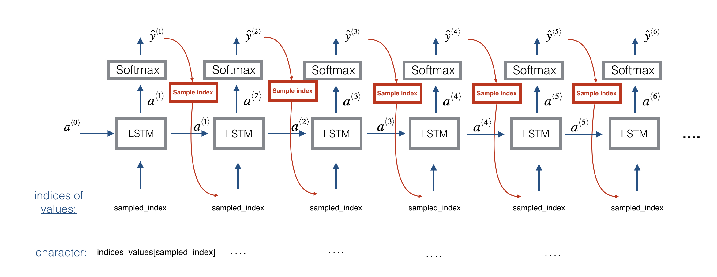
At each step of sampling, you will:
- Take as input the activation '
a' and cell state 'c' from the previous state of the LSTM. - Forward propagate by one step.
- Get a new output activation as well as cell state.
- The new activation '
a' can then be used to generate the output using the fully connected layer,densor.
Initialization
- We will initialize the following to be zeros:
x0- hidden state
a0 - cell state
c0
Exercise:
-
Implement the function below to sample a sequence of musical values.
-
Here are some of the key steps you'll need to implement inside the for-loop that generates the (T_y) output characters:
-
Step 2.A: Use
LSTM_Cell, which takes in the input layer, as well as the previous step's 'c' and 'a' to generate the current step's 'c' and 'a'.
next_hidden_state, _, next_cell_state = LSTM_cell(input_x, initial_state=[previous_hidden_state, previous_cell_state])
-
Choose the appropriate variables for the input_x, hidden_state, and cell_state
-
Step 2.B: Compute the output by applying
densorto compute a softmax on 'a' to get the output for the current step. -
Step 2.C: Append the output to the list
outputs. -
Step 2.D: Sample x to be the one-hot version of '
out'. -
This allows you to pass it to the next LSTM's step.
-
We have provided the definition of
one_hot(x)in the 'music_utils.py' file and imported it.
Here is the definition ofone_hot
def one_hot(x):
    x = K.argmax(x)
    x = tf.one_hot(indices=x, depth=78)
    x = RepeatVector(1)(x)
    return x
Here is what the one_hot function is doing:
- argmax: within the vector
x, find the position with the maximum value and return the index of that position.- For example: argmax of [-1,0,1] finds that 1 is the maximum value, and returns the index position, which is 2. Read the documentation for keras.argmax.
- one_hot: takes a list of indices and the depth of the one-hot vector (number of categories, which is 78 in this assignment). It converts each index into the one-hot vector representation. For instance, if the indices is [2], and the depth is 5, then the one-hot vector returned is [0,0,1,0,0]. Check out the documentation for tf.one_hot for more examples and explanations.
- RepeatVector(n): This takes a vector and duplicates it
ntimes. Notice that we had it repeat 1 time. This may seem like it's not doing anything. If you look at the documentation for RepeatVector, you'll notice that if x is a vector with dimension (m,5) and it gets passed intoRepeatVector(1), then the output is (m,1,5). In other words, it adds an additional dimension (of length 1) to the resulting vector. - Apply the custom one_hot encoding using the Lambda layer. You saw earlier that the Lambda layer can be used like this:
result = Lambda(lambda x: x + 1)(input_var)
If you pre-define a function, you can do the same thing:
def add_one(x)
    return x + 1

# use the add_one function inside of the Lambda function
result = Lambda(add_one)(input_var)
Step 3: Inference Model:
This is how to use the Keras Model.
model = Model(inputs=[input_x, initial_hidden_state, initial_cell_state], outputs=the_outputs)
- Choose the appropriate variables for the input tensor, hidden state, cell state, and output.
- Hint: the inputs to the model are the initial inputs and states.
# GRADED FUNCTION: music_inference_model

def music_inference_model(LSTM_cell, densor, n_values = 78, n_a = 64, Ty = 100):
    """
    Uses the trained "LSTM_cell" and "densor" from model() to generate a sequence of values.

    Arguments:
        LSTM_cell -- the trained "LSTM_cell" from model(), Keras layer object
        densor -- the trained "densor" from model(), Keras layer object
        n_values -- integer, number of unique values
        n_a -- number of units in the LSTM_cell
        Ty -- integer, number of time steps to generate

    Returns:
        inference_model -- Keras model instance
    """

    # Define the input of your model with a shape
    x0 = Input(shape=(1, n_values))

    # Define s0, initial hidden state for the decoder LSTM
    a0 = Input(shape=(n_a,), name='a0')
    c0 = Input(shape=(n_a,), name='c0')
    a = a0
    c = c0
    x = x0

    ### START CODE HERE ###
    # Step 1: Create an empty list of "outputs" to later store your predicted values (≈1 line)
    outputs = []

    # Step 2: Loop over Ty and generate a value at every time step
    for t in range(Ty):

        # Step 2.A: Perform one step of LSTM_cell (≈1 line)
        a, _, c = LSTM_cell(inputs=x, initial_state=[a, c])

        # Step 2.B: Apply Dense layer to the hidden state output of the LSTM_cell (≈1 line)
        out = densor(a)

        # Step 2.C: Append the prediction "out" to "outputs". out.shape = (None, 78) (≈1 line)
        outputs.append(out)

        # Step 2.D:
        # Select the next value according to "out",
        # Set "x" to be the one-hot representation of the selected value
        # See instructions above.
        x = Lambda(one_hot)(out)

    # Step 3: Create model instance with the correct "inputs" and "outputs" (≈1 line)
    inference_model = Model(inputs=[x0, a0, c0], outputs=outputs)

    ### END CODE HERE ###

    return inference_model
Run the cell below to define your inference model. This model is hard coded to generate 50 values.
inference_model = music_inference_model(LSTM_cell, densor, n_values = 78, n_a = 64, Ty = 50)
# Check the inference model
inference_model.summary()
____________________________________________________________________________________________________
Layer (type)                     Output Shape          Param #     Connected to
====================================================================================================
input_24 (InputLayer)            (None, 1, 78)         0
____________________________________________________________________________________________________
a0 (InputLayer)                  (None, 64)            0
____________________________________________________________________________________________________
c0 (InputLayer)                  (None, 64)            0
____________________________________________________________________________________________________
lstm_1 (LSTM)                    multiple              36608       input_24[0][0]
                                                                   a0[0][0]
                                                                   c0[0][0]
                                                                   lambda_332[0][0]
... ... ...
____________________________________________________________________________________________________
lambda_380 (Lambda)              (None, 1, 78)         0           dense_1[808][0]
====================================================================================================
Total params: 41,678
Trainable params: 41,678
Non-trainable params: 0
____________________________________________________________________________________________________
Initialize inference model
The following code creates the zero-valued vectors you will use to initialize x and the LSTM state variables a and c.
x_initializer = np.zeros((1, 1, 78))
a_initializer = np.zeros((1, n_a))
c_initializer = np.zeros((1, n_a))
Exercise: Implement predict_and_sample().
- This function takes many arguments including the inputs [x_initializer, a_initializer, c_initializer].
- In order to predict the output corresponding to this input, you will need to carry-out 3 steps:
Step 1
- Use your inference model to predict an output given your set of inputs. The output
predshould be a list of length (T_y) where each element is a numpy-array of shape (1, n_values).
inference_model.predict([input_x_init, hidden_state_init, cell_state_init])
* Choose the appropriate input arguments to `predict` from the input arguments of this `predict_and_sample` function.
Step 2
- Convert
predinto a numpy array of (T_y) indices.- Each index is computed by taking the
argmaxof an element of thepredlist. - Use numpy.argmax.
- Set the
axisparameter.- Remember that the shape of the prediction is ((m, T_{y}, n_{values}))
- Each index is computed by taking the
Step 3
- Convert the indices into their one-hot vector representations.
- Use to_categorical.
- Set the
num_classesparameter. Note that for grading purposes: you'll need to either:- Use a dimension from the given parameters of
predict_and_sample()(for example, one of the dimensions of x_initializer has the value for the number of distinct classes). - Or just hard code the number of distinct classes (will pass the grader as well).
- Note that using a global variable such as n_values will not work for grading purposes.
- Use a dimension from the given parameters of
# GRADED FUNCTION: predict_and_sample

def predict_and_sample(inference_model, x_initializer = x_initializer, a_initializer = a_initializer,
                       c_initializer = c_initializer):
    """
    Predicts the next value of values using the inference model.

    Arguments:
        inference_model -- Keras model instance for inference time
        x_initializer -- numpy array of shape (1, 1, 78), one-hot vector initializing the values generation
        a_initializer -- numpy array of shape (1, n_a), initializing the hidden state of the LSTM_cell
        c_initializer -- numpy array of shape (1, n_a), initializing the cell state of the LSTM_cel

    Returns:
        results -- numpy-array of shape (Ty, 78), matrix of one-hot vectors representing the values generated
        indices -- numpy-array of shape (Ty, 1), matrix of indices representing the values generated
    """

    ### START CODE HERE ###
    # Step 1: Use your inference model to predict an output sequence given x_initializer, a_initializer and c_initializer.
    pred = inference_model.predict([x_initializer, a_initializer, c_initializer])
    # Step 2: Convert "pred" into an np.array() of indices with the maximum probabilities
    indices = np.argmax(pred, axis=2)
    # Step 3: Convert indices to one-hot vectors, the shape of the results should be (Ty, n_values)
    results = to_categorical(indices, num_classes=n_values)
    ### END CODE HERE ###

    return results, indices
results, indices = predict_and_sample(inference_model, x_initializer, a_initializer, c_initializer)
print("np.argmax(results[12]) =", np.argmax(results[12]))
print("np.argmax(results[17]) =", np.argmax(results[17]))
print("list(indices[12:18]) =", list(indices[12:18]))
np.argmax(results[12]) = 56
np.argmax(results[17]) = 3
list(indices[12:18]) = [array([56]), array([15]), array([56]), array([47]), array([17]), array([3])]
Expected (Approximate) Output :
- Your results may likely differ because Keras' results are not completely predictable.
- However, if you have trained your LSTM_cell with model.fit() for exactly 100 epochs as described above:
- You should very likely observe a sequence of indices that are not all identical.
- Moreover, you should observe that:
- np.argmax(results[12]) is the first element of list(indices[12:18])
- and np.argmax(results[17]) is the last element of list(indices[12:18]).
3.3 - Generate music
Finally, you are ready to generate music. Your RNN generates a sequence of values. The following code generates music by first calling your predict_and_sample() function. These values are then post-processed into musical chords (meaning that multiple values or notes can be played at the same time).
Most computational music algorithms use some post-processing because it is difficult to generate music that sounds good without such post-processing. The post-processing does things such as clean up the generated audio by making sure the same sound is not repeated too many times, that two successive notes are not too far from each other in pitch, and so on. One could argue that a lot of these post-processing steps are hacks; also, a lot of the music generation literature has also focused on hand-crafting post-processors, and a lot of the output quality depends on the quality of the post-processing and not just the quality of the RNN. But this post-processing does make a huge difference, so let's use it in our implementation as well.
Let's make some music!
Run the following cell to generate music and record it into your out_stream. This can take a couple of minutes.
out_stream = generate_music(inference_model)
Predicting new values for different set of chords.
Generated 51 sounds using the predicted values for the set of chords ("1") and after pruning
Generated 51 sounds using the predicted values for the set of chords ("2") and after pruning
Generated 51 sounds using the predicted values for the set of chords ("3") and after pruning
Generated 50 sounds using the predicted values for the set of chords ("4") and after pruning
Generated 51 sounds using the predicted values for the set of chords ("5") and after pruning
Your generated music is saved in output/my_music.midi
To listen to your music, click File->Open... Then go to "output/" and download "my_music.midi". Either play it on your computer with an application that can read midi files if you have one, or use one of the free online "MIDI to mp3" conversion tools to convert this to mp3.
As a reference, here is a 30 second audio clip we generated using this algorithm.
IPython.display.Audio('./data/30s_trained_model.mp3')
Congratulations!
You have come to the end of the notebook.
What you should remember
- A sequence model can be used to generate musical values, which are then post-processed into midi music.
- Fairly similar models can be used to generate dinosaur names or to generate music, with the major difference being the input fed to the model.
- In Keras, sequence generation involves defining layers with shared weights, which are then repeated for the different time steps (1, ldots, T_x).
Congratulations on completing this assignment and generating a jazz solo!
References
The ideas presented in this notebook came primarily from three computational music papers cited below. The implementation here also took significant inspiration and used many components from Ji-Sung Kim's GitHub repository.
- Ji-Sung Kim, 2016, deepjazz
- Jon Gillick, Kevin Tang and Robert Keller, 2009. Learning Jazz Grammars
- Robert Keller and David Morrison, 2007, A Grammatical Approach to Automatic Improvisation
- François Pachet, 1999, Surprising Harmonies
We're also grateful to François Germain for valuable feedback.