from __future__ import print_function
import tensorflow as tf
import numpy
import matplotlib.pyplot as plt
rng = numpy.random
# Parameters
# 模型的超参数
# 学习率
learning_rate = 0.01
# 训练迭代次数
training_epochs = 1000
display_step = 50
# 模拟生成的一段训练数据
# Training Data
train_X = numpy.asarray([3.3, 4.4, 5.5, 6.71, 6.93, 4.168, 9.779, 6.182, 7.59, 2.167,
7.042, 10.791, 5.313, 7.997, 5.654, 9.27, 3.1])
train_Y = numpy.asarray([1.7, 2.76, 2.09, 3.19, 1.694, 1.573, 3.366, 2.596, 2.53, 1.221,
2.827, 3.465, 1.65, 2.904, 2.42, 2.94, 1.3])
# train_X的长度
n_samples = train_X.shape[0]
# 占位符
X = tf.placeholder("float")
Y = tf.placeholder("float")
# 随机权重和偏置
W = tf.Variable(rng.randn(), name="weight")
b = tf.Variable(rng.randn(), name="bias")
# 决策函数
pred = tf.add(tf.multiply(X, W), b)
# 损失函数
cost = tf.reduce_sum(tf.pow(pred - Y, 2)) / (2 * n_samples)
# 优化方法
optimizer = tf.train.GradientDescentOptimizer(learning_rate).minimize(cost)
# 模型参数初始化
init = tf.initialize_all_variables()
# 创建计算图
with tf.Session() as sess:
sess.run(init)
# 迭代训练循环
for epoch in range(training_epochs):
for (x, y) in zip(train_X, train_Y):
# feed_dict将数据放入模型
sess.run(optimizer, feed_dict={X: x, Y: y})
# 每隔50次显示一下损失函数的值
if (epoch + 1) % display_step == 0:
c = sess.run(cost, feed_dict={X: train_X, Y: train_Y})
print("Epoch:", '%04d' % (epoch + 1), "cost=", "{:.9f}".format(c),
"W=", sess.run(W), "b=", sess.run(b))
###############
print("Optimization Finished!")
# 训练结束时,显示最终损失函数的值
training_cost = sess.run(cost, feed_dict={X: train_X, Y: train_Y})
print("Training cost=", training_cost, "W=", sess.run(W), "b=", sess.run(b), '
')
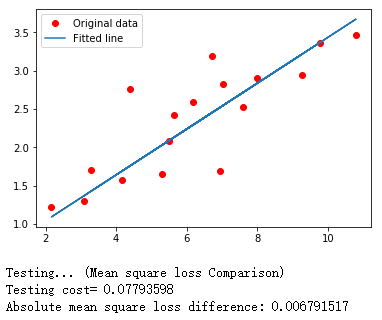
# 用matplotlib生成一幅图
plt.plot(train_X, train_Y, 'ro', label='Original data')
plt.plot(train_X, sess.run(W) * train_X + sess.run(b), label='Fitted line')
plt.legend()
plt.show()
# 生成一段测试文件
test_X = numpy.asarray([6.83, 4.668, 8.9, 7.91, 5.7, 8.7, 3.1, 2.1])
test_Y = numpy.asarray([1.84, 2.273, 3.2, 2.831, 2.92, 3.24, 1.35, 1.03])
print("Testing... (Mean square loss Comparison)")
# 用训练好的参数根据test_x预测对应的y
testing_cost = sess.run(tf.reduce_sum(tf.pow(pred - Y, 2)) / (2 * test_X.shape[0]),
feed_dict={X: test_X, Y: test_Y})
print("Testing cost=", testing_cost)
# 比较一下训练的损失函数值和测试损失函数值
print("Absolute mean square loss difference:", abs(training_cost - testing_cost))
plt.plot(test_X, test_Y, 'bo', label='Testing data')
plt.plot(train_X, sess.run(W) * train_X + sess.run(b), label='Fitted line')
plt.legend()
plt.show()
结果
Epoch: 0050 cost= 0.157032505 W= 0.4078232 b= -0.33682635
Epoch: 0100 cost= 0.147781506 W= 0.3984126 b= -0.2691267
Epoch: 0150 cost= 0.139598981 W= 0.3895616 b= -0.20545363
Epoch: 0200 cost= 0.132361546 W= 0.38123706 b= -0.14556733
Epoch: 0250 cost= 0.125960082 W= 0.37340772 b= -0.08924285
Epoch: 0300 cost= 0.120298132 W= 0.3660438 b= -0.03626821
Epoch: 0350 cost= 0.115290195 W= 0.35911795 b= 0.013555876
Epoch: 0400 cost= 0.110860869 W= 0.352604 b= 0.060416616
Epoch: 0450 cost= 0.106943212 W= 0.34647754 b= 0.10449031
Epoch: 0500 cost= 0.103478260 W= 0.34071538 b= 0.1459427
Epoch: 0550 cost= 0.100413688 W= 0.33529598 b= 0.18492968
Epoch: 0600 cost= 0.097703241 W= 0.33019873 b= 0.22159818
Epoch: 0650 cost= 0.095306024 W= 0.32540485 b= 0.25608563
Epoch: 0700 cost= 0.093185902 W= 0.320896 b= 0.28852215
Epoch: 0750 cost= 0.091310821 W= 0.31665528 b= 0.31902957
Epoch: 0800 cost= 0.089652546 W= 0.3126668 b= 0.347722
Epoch: 0850 cost= 0.088185944 W= 0.30891564 b= 0.37470827
Epoch: 0900 cost= 0.086888909 W= 0.30538744 b= 0.40008995
Epoch: 0950 cost= 0.085741922 W= 0.30206922 b= 0.42396098
Epoch: 1000 cost= 0.084727496 W= 0.29894808 b= 0.44641364
Optimization Finished!
Training cost= 0.084727496 W= 0.29894808 b= 0.44641364