高斯核函数的代码体现

直观理解高斯核函数
scikit-learn 中的 RBF 核

直观理解高斯核函数

import numpy as np
import matplotlib.pyplot as plt
 
x = np.arange(-4, 5, 1) 
x
# array([-4, -3, -2, -1,  0,  1,  2,  3,  4])
 
y = np.array((x >= -2) & (x <= 2), dtype='int')
y
# array([0, 0, 1, 1, 1, 1, 1, 0, 0])
 
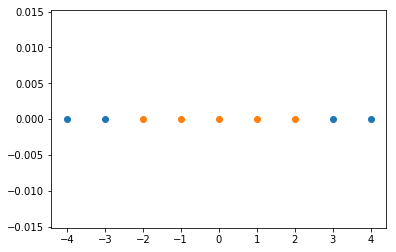
plt.scatter(x[y==0], [0]*len(x[y==0]))
plt.scatter(x[y==1], [0]*len(x[y==1]))
plt.show()

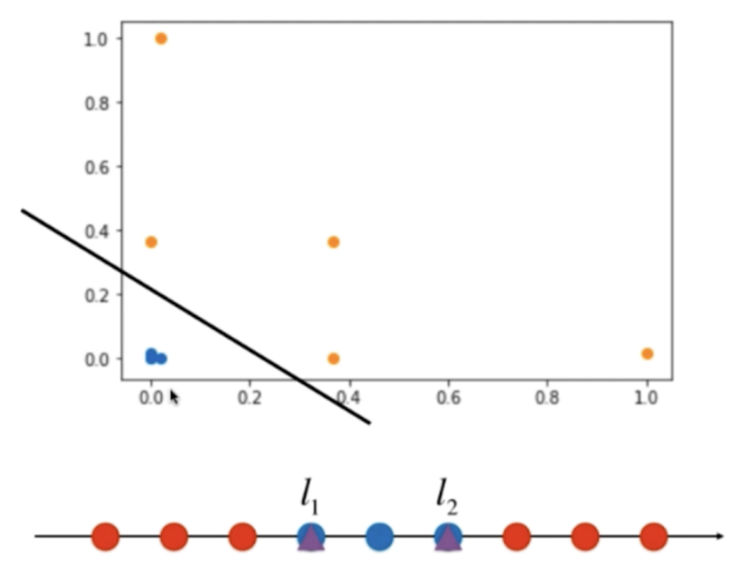
使用高斯核函数，让数据可分

def gaussian(x, l):
    gamma = 1.0
    return np.exp(-gamma * (x-l)**2)
 
 
l1, l2 = -1, 1

X_new = np.empty((len(x), 2))
for i, data in enumerate(x):
    X_new[i, 0] = gaussian(data, l1)
    X_new[i, 1] = gaussian(data, l2)
 
 
plt.scatter(X_new[y==0,0], X_new[y==0,1])
plt.scatter(X_new[y==1,0], X_new[y==1,1])
plt.show()

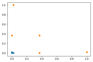
这样数据就变成线性可分了

scikit-learn 中的 RBF 核

查看 gamma 的影响

import numpy as np
import matplotlib.pyplot as plt

from sklearn import datasets

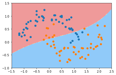
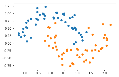
X, y = datasets.make_moons(noise=0.15, random_state=666)

plt.scatter(X[y==0,0], X[y==0,1])
plt.scatter(X[y==1,0], X[y==1,1])
plt.show()

from sklearn.preprocessing import StandardScaler
from sklearn.pipeline import Pipeline
from sklearn.svm import SVC

def RBFKernelSVC(gamma):
    return Pipeline([
        ("std_scaler", StandardScaler()),
        ("svc", SVC(kernel="rbf", gamma=gamma))
    ])

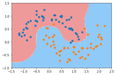
svc = RBFKernelSVC(gamma=1)
svc.fit(X, y)

Pipeline(steps=[('std_scaler', StandardScaler(copy=True, with_mean=True, with_std=True)), ('svc', SVC(C=1.0, cache_size=200, class_weight=None, coef0=0.0,
  decision_function_shape=None, degree=3, gamma=1, kernel='rbf',
  max_iter=-1, probability=False, random_state=None, shrinking=True,
  tol=0.001, verbose=False))])

def plot_decision_boundary(model, axis):
    
    x0, x1 = np.meshgrid(
        np.linspace(axis[0], axis[1], int((axis[1]-axis[0])*100)).reshape(-1, 1),
        np.linspace(axis[2], axis[3], int((axis[3]-axis[2])*100)).reshape(-1, 1),
    )
    X_new = np.c_[x0.ravel(), x1.ravel()]

    y_predict = model.predict(X_new)
    zz = y_predict.reshape(x0.shape)

    from matplotlib.colors import ListedColormap
    custom_cmap = ListedColormap(['#EF9A9A','#FFF59D','#90CAF9'])
    
    plt.contourf(x0, x1, zz, linewidth=5, cmap=custom_cmap)

plot_decision_boundary(svc, axis=[-1.5, 2.5, -1.0, 1.5])
plt.scatter(X[y==0,0], X[y==0,1])
plt.scatter(X[y==1,0], X[y==1,1])
plt.show()

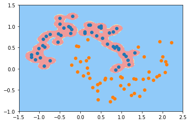
gamma=100

过拟合

svc_gamma100 = RBFKernelSVC(gamma=100)
svc_gamma100.fit(X, y)

Pipeline(steps=[('std_scaler', StandardScaler(copy=True, with_mean=True, with_std=True)), ('svc', SVC(C=1.0, cache_size=200, class_weight=None, coef0=0.0,
  decision_function_shape=None, degree=3, gamma=100, kernel='rbf',
  max_iter=-1, probability=False, random_state=None, shrinking=True,
  tol=0.001, verbose=False))])

plot_decision_boundary(svc_gamma100, axis=[-1.5, 2.5, -1.0, 1.5])
plt.scatter(X[y==0,0], X[y==0,1])
plt.scatter(X[y==1,0], X[y==1,1])
plt.show()

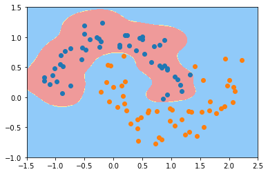
gamma=10

svc_gamma10 = RBFKernelSVC(gamma=10)
svc_gamma10.fit(X, y)

Pipeline(steps=[('std_scaler', StandardScaler(copy=True, with_mean=True, with_std=True)), ('svc', SVC(C=1.0, cache_size=200, class_weight=None, coef0=0.0,
  decision_function_shape=None, degree=3, gamma=10, kernel='rbf',
  max_iter=-1, probability=False, random_state=None, shrinking=True,
  tol=0.001, verbose=False))])

plot_decision_boundary(svc_gamma10, axis=[-1.5, 2.5, -1.0, 1.5])
plt.scatter(X[y==0,0], X[y==0,1])
plt.scatter(X[y==1,0], X[y==1,1])
plt.show()

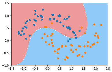
gamma=0.5

svc_gamma05 = RBFKernelSVC(gamma=0.5)
svc_gamma05.fit(X, y)

Pipeline(steps=[('std_scaler', StandardScaler(copy=True, with_mean=True, with_std=True)), ('svc', SVC(C=1.0, cache_size=200, class_weight=None, coef0=0.0,
  decision_function_shape=None, degree=3, gamma=0.5, kernel='rbf',
  max_iter=-1, probability=False, random_state=None, shrinking=True,
  tol=0.001, verbose=False))])

plot_decision_boundary(svc_gamma05, axis=[-1.5, 2.5, -1.0, 1.5])
plt.scatter(X[y==0,0], X[y==0,1])
plt.scatter(X[y==1,0], X[y==1,1])
plt.show()

gamma=0.1

跟线性的决策边界差不多；

欠拟合

svc_gamma01 = RBFKernelSVC(gamma=0.1)
svc_gamma01.fit(X, y)

Pipeline(steps=[('std_scaler', StandardScaler(copy=True, with_mean=True, with_std=True)), ('svc', SVC(C=1.0, cache_size=200, class_weight=None, coef0=0.0,
  decision_function_shape=None, degree=3, gamma=0.1, kernel='rbf',
  max_iter=-1, probability=False, random_state=None, shrinking=True,
  tol=0.001, verbose=False))])

plot_decision_boundary(svc_gamma01, axis=[-1.5, 2.5, -1.0, 1.5])
plt.scatter(X[y==0,0], X[y==0,1])
plt.scatter(X[y==1,0], X[y==1,1])
plt.show()