决策树是一种基本的分类与回归方法,称之为"树",是因为决策树模型呈树形结构。本小结主要讨论用于分类的决策树,那么决策树是如何从一大堆无序的数据特征中找出有序的规则,并构建决策树呢?
1 信息论知识
回答上面的问题,将一堆无序的数据变得更有序,一种方法是使用信息论度量信息。在划分数据前后,使用信息论量化度量信息的内容。在划分数据集前后,信息发生的变化称为信息增益,计算每个特征划分数据集获得的信息增益,获得信息增益最高的特征就是最好的选择。评测哪种数据划分方式是最好的数据划分前,先计算信息增益。
大家都知道一个事实,一件事发生的概率越小,它蕴含的信息量就越大。如果待分类的食物可能划分在多个分类中,则衡量信息量的表达式为:
其中(p(x_{i}))是选择该分类的概率。
信息熵是所有类别所有可能值保护的信息量的期望:
表示事件(X)发生的不确定度,(n)表示(X)的(n)种离散取值,也就是分类的数目。
2 决策树ID3算法
前面给出了一个事件(变量)X的熵,推广到多个事件的联合熵,给出事件X和Y的联合熵表达式: (H(X,Y)=-sum_{i=1}^{n}p(x_{i},y_{i})logp(x_{i},y_{i}))
条件熵表达式:(H(X|Y)=-sum_{i=1}^{n}p(x_{i},y_{i})logp(x_{i}|y_{i})=sum_{j=1}^{n}p(y_{j})H(X|y_{j})) 度量在Y已知情况下X剩下的不确定性
另外,(H(X)-H(X|Y)) 度量X在Y已知情况下不确定性减少的程度,信息论中称为互信息(I(X,Y)),在决策树ID3算法中称为信息增益,ID3算法中用信息增益衡量使用当前特征
对样本划分的效果,其中信息增益越大,表示当前特征更适合用来分类。
信息增益的算法
输入: 训练数据集(D)和特征(A)
输出: 特征(A)对训练数据集(D)的信息增益(g(D,A))
step1: 计算数据集(D)的熵(H(D)) $$H(D)=-sum_{k=1}^{K}frac{|C_{k}|}{|D|}log_{2}frac{|C_{k}|}{|D|}$$ 其中(K)表示类别的个数,(|C_{k}|)表示属于类(C_{k})的个数,(|D|)表示样本个数
step2: 计算特征(A)对数据集(D)的条件熵(H(D|A)) $$H(D|A)=sum_{i=1}{n}frac{|D_{i}|}{|D|}H(D_{i})=-sum_{i=1}{n}frac{|D_{i}|}{|D|}sum_{k=1}^{K}frac{|D_{ik}|}{|D_{i}|}log_{2}frac{|D_{ik}|}{|D_{i}|}$$ 其中(n)表示特征(A)取值的个数,特征(A)取值将数据集(D)划分为(n)个子集$D_{1},D_{2},cdots,D_{n} $ ,(|D_{i}|) 表示(D_{i})样本的个数, (K)表示特征(A)的样本输出类别的个数,(D_{ik})表示子集(D_{i})中属于类(C_{k})的个数,(|D_{ik}|)表示(D_{ik})的样本个数
step3: 计算信息增益 $$g(D,A)=H(D)-H(D|A)$$
举例,给表中所给的训练数据集(D),根据信息增益准则选择最优特征
首先计算熵据集(D)的熵(H(D)) $$H(D)=-frac{9}{15}log_{2}frac{9}{15}-frac{6}{15}log_{2}frac{6}{15}=0.971$$ 数据集(D)有15个样本,输出类别只有"是"和"否"两类, 其中9个输出"是",6个输出"否"。
然后计算各特征对数据集(D)的信息增益。分别以(A_{1}),(A_{2}),(A_{3}),(A_{4})表示年龄 有工作 有自己的房子和信贷情况4个特征

最后,比较各特征的信息增益值,由于特征(A_{3})的信息增益值最大,因此选择特征(A_{3})作为最优特征。
ID3算法核心是在决策树各个结点上用信息增益准则选择特征,递归地构建决策树,相当于用极大似然法进行概率模型的选择。
决策树ID3算法
输入: 训练数据集(D),特征集(A),阈值$varepsilon $;
输出: 决策树(T)
step1 若(D)中所有实例属于同一类(C_{k}),则(T)为单结点树,并将类(C_{k})作为该结点的类标记,返回(T);
step2 若(A=Phi),则(T)为单结点树,并将(D)中实例数最大的类(C_{k})作为该结点的类标记,返回(T);
step3 否则计算特征集(A)中各特征对(D)的信息增益,选择信息增益最大的特征(A_{g});
step4 如果(A_{g})的信息增益小于阈值(varepsilon),则置(T)为单结点树,并将(D)中实例数最大的类(C_{k})作为该结点的类标记,返回(T);
step5 否则,对(A_{g})的每一个取值(A_{gi})将对应的样本输出(D)分成不同的类别(D_{i}),每个类别产生一个子节点,对应特征值是(A_{gi}),返回增加了结点的树;
step6 对所有的子结点,以(D_{i})为训练集,以(A-{A_{g}})为特征集,递归调用(1)-(5),得到子树(T_{i}),返回(T_{i}).
3 决策树代码实现
计算给定数据集的香农熵--使用熵划分数据集
from math import log

def calcShannonEnt(dataSet):
    numEntries = len(dataSet)  #计算数据集中实例的总数
    labelCounts = {}  #创建数据字典 其键值是最后一列的数值
    for featVec in dataSet:   #为所有可能分类创建字典
        currentLabel = featVec[-1]
        if currentLabel not in labelCounts.keys():
            labelCounts[currentLabel] = 0  #每个键值记录当前类别出现的次数
        labelCounts[currentLabel] += 1
    shannonEnt = 0.0
    for key in labelCounts:
        prob = float(labelCounts[key])/numEntries   #使用所有类标签的发生频率计算类别出现的概率
        shannonEnt -= prob*log(prob, 2)  #以2为底求对数 统计所有类标签发生的次数
    return shannonEnt
#创建数据集和标签
def createDataSet():
    dataSet = [[1, 1,'yes'],
               [1, 1, 'yes'],
               [1, 0, 'no'],
               [0, 1, 'no'],
               [0, 1, 'no']]
    labels = ['no surfacing', 'flippers']
    return dataSet, labels
#运行效果
myDat, labels = createDataSet()
print(myDat, labels)
#输出
[[1, 1, 'yes'], [1, 1, 'yes'], [1, 0, 'no'], [0, 1, 'no'], [0, 1, 'no']]
['no surfacing', 'flippers']

print(calcShannonEnt(myDat))
#输出
0.9709505944546686  #熵越高,则混合的数据也越多
在数据集中添加更多的分类,观察熵是如何变化的。增加第三个名为maybe的分类,测试熵的变化
myDat, labels = createDataSet()
myDat[0][-1] = 'maybe'
print(myDat, labels)
#输出
[[1, 1, 'maybe'], [1, 1, 'yes'], [1, 0, 'no'], [0, 1, 'no'], [0, 1, 'no']]
['no surfacing', 'flippers']

print(calcShannonEnt(myDat))
#输出
1.3709505944546687  #得到熵 就可以按照获取最大信息增益的方法划分数据集
前面学习了如何度量数据集的无序程度,分类算法除了需要测量信息熵,还需要划分数据集,度量划分数据集的熵,以便判断当前是否正确地划分了数据集。对每个特征划分数据集的结果计算一次信息熵,然后判断按照哪个特征划分数据集是最好的划分方式。
#按照给定特征划分数据集
def splitDataSet(dataSet, axis, value):  #三个参数:待划分数据集 划分数据集的特征 需要返回的特征的值
    retDataSet = []  #创建新的list对象 由于该代码函数在同一数据集上被调用多次 为了不修改原始数据集创建了新的列表对象
    for featVec in dataSet:  #遍历数据集中的每个元素 符合要求的值将其添加到新创建的列表中(注:数据集这个列表中的各个元素也是列表)
        if featVec[axis] == value: #抽取符合条件的数据 即按照某个特征划分数据集时 需要把所有符合要求的元素抽取出来
            reducedFeatVec = featVec[:axis]
            reducedFeatVec.extend(featVec[axis+1:])
            retDataSet.append(reducedFeatVec)
    return retDataSet
#测试splitDataSet()
myDat, labels = createDataSet()
print(myDat)
#输出
[[1, 1, 'yes'], [1, 1, 'yes'], [1, 0, 'no'], [0, 1, 'no'], [0, 1, 'no']]

print(splitDataSet(myDat,0,1))
#输出
[[1, 'yes'], [1, 'yes'], [0, 'no']]

print(splitDataSet(myDat,0,0))
#输出
[[1, 'no'], [1, 'no']]
遍历整个数据集,循环计算香农熵和splitDataSet()函数,找到最好的特征划分方式。熵计算将会告诉我们如何划分数据集是最好的数据组织方式。
#选择最好的数据集划分方式—该函数实现选取特征 划分数据集 计算出最好的划分数据集的特征
def chooseBestFeatureToSplit(dataSet):
    numFeatures = len(dataSet[0]) - 1 #判定当前数据集包含多少特征属性
    baseEntroy = calcShannonEnt(dataSet) #计算整个数据集的原始香农熵 用于与划分完之后的数据集计算的熵值进行比较
    bestInfoGain = 0.0
    bestFeature = -1
    for i in range(numFeatures): #遍历数据集中的所有特征
        featureList = [example[i] for example in dataSet] #使用列表推到创建新的列表 将数据中所有第i个特征值写入这个新list中
        uniqueVals = set(featureList)  #得到唯一的分类标签列表
        newEntropy = 0.0
        for value in uniqueVals: #计算每种划分方式的信息熵 遍历当前特征中的所有唯一属性值 对每个特征划分一次数据集
            subDataSet = splitDataSet(dataSet, i, value)
            prob = len(subDataSet)/float(len(dataSet)) #计算数据集的新熵值
            newEntropy += prob*calcShannonEnt(subDataSet) #对所有唯一特征值得到的熵求和
        infoGain = baseEntroy - newEntropy  #信息增益是熵的减少或者是数据无序度的减少
        if (infoGain > bestInfoGain): #计算最好的信息增益 比较所有特征中的信息增益
            bestInfoGain = infoGain
            bestFeature = i
    return bestFeature #返回最好特征划分的索引值
#测试
myDat, labels = createDataSet()
print(chooseBestFeatureToSplit(myDat))
#输出 第0个特征是最好的用于划分数据集的特征
0

print(myDat)
#输出
[[1, 1, 'yes'], [1, 1, 'yes'], [1, 0, 'no'], [0, 1, 'no'], [0, 1, 'no']]
介绍了如何度量数据集的信息熵,如何有效地划分数据集,下面将介绍如何将这些函数功能放在一起,构建决策树。
递归构建决策树
#采用多数表决的方法决定叶子节点的分类
import operator
def majorityCnt(classList): #classList分类名称的列表
    classCount = {}  #创建键值为classList中唯一值的数据字典 字典对象存储classList中每个类标签出现的频率
    for vote in classList:
        if vote not in classCount.keys():
            classCount[vote] = 0
        classCount[vote] += 1
    sortedClassCount = sorted(classCount.items(),key=operator.itemgetter(1),reverse=True) #operator操作键值排序字典 降序排序
    return sortedClassCount[0][0] #返回出现次数最多的分类名称
#创建树的函数代码
def createTree(dataSet, labels):
    classList = [example[-1] for example in dataSet] #classList列表 包含数据集的所有类标签
    if classList.count(classList[0]) == len(classList): #类别完全相同则停止划分  递归函数的第一个停止条件 所有的类标签完全相同
        return classList[0] #直接返回该类标签

    if len(dataSet[0]) == 1: #遍历完所有特征时返回出现次数最多的 递归函数的第二个停止条件 使用完所有特征仍不能将数据集划分成仅包含唯一类别的分组
        return majorityCnt(classList) #该停止条件无法返回唯一的类标签 这里返回出现次数最多的类别

    bestFeat = chooseBestFeatureToSplit(dataSet)
    bestFeatLabel = labels[bestFeat]
    myTree = {bestFeatLabel: {}} #创建树 使用字典类型存储树的所有信息

    del (labels[bestFeat])
    featValues = [example[bestFeat] for example in dataSet] #得到列表包含的所有属性值 遍历当前选择特征包含的所有属性值
    uniqueVals = set(featValues)

    for value in uniqueVals:
        subLabels = labels[:] #复制类标签 确保每次调用createTree()时不改变原始列表的内容
        myTree[bestFeatLabel][value] = createTree(splitDataSet(dataSet, bestFeat, value),subLabels) #在每个数据集划分上递归调用createTree()得到的返回值插入到字典myTree
    return myTree
#测试
myDat, labels = createDataSet()
myTree = createTree(myDat, labels)
print(myTree)
#输出
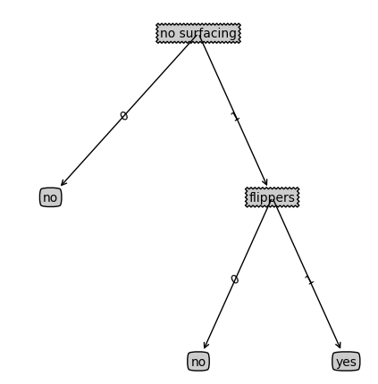
{'no surfacing': {0: 'no', 1: {'flippers': {0: 'no', 1: 'yes'}}}}
测试算法:使用决策树执行分类
def classify(inputTree,featLabels,testVec):
    firstStr = inputTree.keys()[0]
    secondDict = inputTree[firstStr]
    featIndex = featLabels.index(firstStr)
    key = testVec[featIndex]
    valueOfFeat = secondDict[key]
    if isinstance(valueOfFeat, dict):
        classLabel = classify(valueOfFeat, featLabels, testVec)
    else: classLabel = valueOfFeat
    return classLabel
绘图部分
''' Created on Oct 14, 2010@author: Peter Harrington
'''
import matplotlib.pyplot as pltdecisionNode = dict(boxstyle="sawtooth", fc="0.8")
leafNode = dict(boxstyle="round4", fc="0.8")
arrow_args = dict(arrowstyle="<-")def getNumLeafs(myTree):
numLeafs = 0
firstStr = myTree.keys()[0]
secondDict = myTree[firstStr]
for key in secondDict.keys():
if type(secondDict[key]).name=='dict':#test to see if the nodes are dictonaires, if not they are leaf nodes
numLeafs += getNumLeafs(secondDict[key])
else: numLeafs +=1
return numLeafsdef getTreeDepth(myTree):
maxDepth = 0
firstStr = myTree.keys()[0]
secondDict = myTree[firstStr]
for key in secondDict.keys():
if type(secondDict[key]).name=='dict':#test to see if the nodes are dictonaires, if not they are leaf nodes
thisDepth = 1 + getTreeDepth(secondDict[key])
else: thisDepth = 1
if thisDepth > maxDepth: maxDepth = thisDepth
return maxDepthdef plotNode(nodeTxt, centerPt, parentPt, nodeType):
createPlot.ax1.annotate(nodeTxt, xy=parentPt, xycoords='axes fraction',
xytext=centerPt, textcoords='axes fraction',
va="center", ha="center", bbox=nodeType, arrowprops=arrow_args )def plotMidText(cntrPt, parentPt, txtString):
xMid = (parentPt[0]-cntrPt[0])/2.0 + cntrPt[0]
yMid = (parentPt[1]-cntrPt[1])/2.0 + cntrPt[1]
createPlot.ax1.text(xMid, yMid, txtString, va="center", ha="center", rotation=30)def plotTree(myTree, parentPt, nodeTxt):#if the first key tells you what feat was split on
numLeafs = getNumLeafs(myTree) #this determines the x width of this tree
depth = getTreeDepth(myTree)
firstStr = myTree.keys()[0] #the text label for this node should be this
cntrPt = (plotTree.xOff + (1.0 + float(numLeafs))/2.0/plotTree.totalW, plotTree.yOff)
plotMidText(cntrPt, parentPt, nodeTxt)
plotNode(firstStr, cntrPt, parentPt, decisionNode)
secondDict = myTree[firstStr]
plotTree.yOff = plotTree.yOff - 1.0/plotTree.totalD
for key in secondDict.keys():
if type(secondDict[key]).name=='dict':#test to see if the nodes are dictonaires, if not they are leaf nodes
plotTree(secondDict[key],cntrPt,str(key)) #recursion
else: #it's a leaf node print the leaf node
plotTree.xOff = plotTree.xOff + 1.0/plotTree.totalW
plotNode(secondDict[key], (plotTree.xOff, plotTree.yOff), cntrPt, leafNode)
plotMidText((plotTree.xOff, plotTree.yOff), cntrPt, str(key))
plotTree.yOff = plotTree.yOff + 1.0/plotTree.totalDif you do get a dictonary you know it's a tree, and the first element will be another dict
def createPlot(inTree):
fig = plt.figure(1, facecolor='white')
fig.clf()
axprops = dict(xticks=[], yticks=[])
createPlot.ax1 = plt.subplot(111, frameon=False, **axprops) #no ticks
#createPlot.ax1 = plt.subplot(111, frameon=False) #ticks for demo puropses
plotTree.totalW = float(getNumLeafs(inTree))
plotTree.totalD = float(getTreeDepth(inTree))
plotTree.xOff = -0.5/plotTree.totalW; plotTree.yOff = 1.0;
plotTree(inTree, (0.5,1.0), '')
plt.show()def createPlot():
fig = plt.figure(1, facecolor='white')
fig.clf()
createPlot.ax1 = plt.subplot(111, frameon=False) #ticks for demo puropses
plotNode('a decision node', (0.5, 0.1), (0.1, 0.5), decisionNode)
plotNode('a leaf node', (0.8, 0.1), (0.3, 0.8), leafNode)
plt.show()
def retrieveTree(i):
listOfTrees =[{'no surfacing': {0: 'no', 1: {'flippers': {0: 'no', 1: 'yes'}}}},
{'no surfacing': {0: 'no', 1: {'flippers': {0: {'head': {0: 'no', 1: 'yes'}}, 1: 'no'}}}}
]
return listOfTrees[i]createPlot(thisTree)
import treePlotter
myDat, labels = createDataSet()
print(labels)
#输出
['no surfacing', 'flippers']
myTree = treePlotter.retrieveTree(0)
print(myTree)
#输出
{'no surfacing': {0: 'no', 1: {'flippers': {0: 'no', 1: 'yes'}}}}
print(classify(myTree, labels, [1, 0]))
#输出
'no'
print(classify(myTree, labels, [1, 1]))
#输出
'yes'
使用算法:决策树的存储
#使用pickle模块存储决策树
def storeTree(inputTree,filename):
    import pickle
    fw = open(filename,'wb')
    pickle.dump(inputTree,fw)
    fw.close()

def grabTree(filename):
    import pickle
    fr = open(filename, 'rb')
    return pickle.load(fr)
storeTree(myTree, 'classifierStorage.txt')
print(grabTree('classifierStorage.txt'))
#输出
{'no surfacing': {0: 'no', 1: {'flippers': {0: 'no', 1: 'yes'}}}}
测试绘制决策树图的函数:
>>> import imp
>>> import trees
>>> imp.reload(trees)
<module 'trees' from 'D:\Python\Mechine_learning\Tree\trees.py'>
>>> import treePlotter
>>> myTree = treePlotter.retrieveTree(0)
>>> treePlotter.createPlot(myTree)
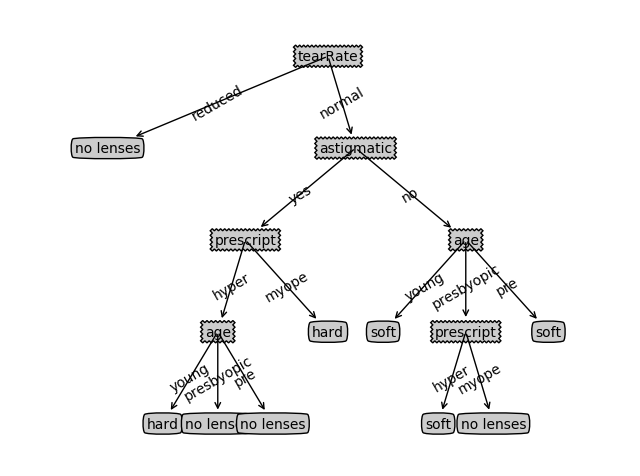
4 使用决策树预测隐形眼镜类型
import treePlotter
fr = open('lenses.txt')
lenses = [inst.strip().split('	') for inst in fr.readlines()]
lensesLabels = ['age', 'prescript', 'astigmatic', 'tearRate']
lensesTree = createTree(lenses, lensesLabels)
print(lensesTree)
#输出
{'tearRate': {'reduced': 'no lenses', 'normal': {'astigmatic': {'no': {'age': {'young': 'soft', 'pre': 'soft', 'presbyopic': {'prescript': {'myope': 'no lenses', 'hyper': 'soft'}}}}, 'yes': {'prescript': {'myope': 'hard', 'hyper': {'age': {'young': 'hard', 'pre': 'no lenses', 'presbyopic': 'no lenses'}}}}}}}}

treePlotter.createPlot(lensesTree)
由ID3算法产生的决策树:
4 ID3算法总结
缺点:信息增益偏向取值较多的特征
原因:当特征的取值较多时,根据此特征划分更容易得到纯度更高的子集,因此划分之后的熵更低,由于划分前的熵是一定的,因此信息增益更大,因此信息增益比较 偏向取值较多的特征。
参考:统计学习方法 机器学习实战 决策树算法原理