1. 详解
STL (Seasonal-Trend decomposition procedure based on Loess) [1] 为时序分解中一种常见的算法,基于LOESS将某时刻的数据(Y_v)分解为趋势分量(trend component)、周期分量(seasonal component)和余项(remainder component):
STL分为内循环(inner loop)与外循环(outer loop),其中内循环主要做了趋势拟合与周期分量的计算。假定(T_v^{(k)})、(S_v{(k)})为内循环中第k-1次pass结束时的趋势分量、周期分量,初始时(T_v^{(k)} = 0);并有以下参数:
- (n_{(i)})内层循环数,
- (n_{(o)})外层循环数,
- (n_{(p)})为一个周期的样本数,
- (n_{(s)})为Step 2中LOESS平滑参数,
- (n_{(l)})为Step 3中LOESS平滑参数,
- (n_{(t)})为Step 6中LOESS平滑参数。
每个周期相同位置的样本点组成一个子序列(subseries),容易知道这样的子序列共有共有(n_(p))个,我们称其为cycle-subseries。内循环主要分为以下6个步骤:
- Step 1: 去趋势(Detrending),减去上一轮结果的趋势分量,(Y_v - T_v^{(k)});
- Step 2: 周期子序列平滑(Cycle-subseries smoothing),用LOESS ((q=n_{n(s)}), (d=1))对每个子序列做回归,并向前向后各延展一个周期;平滑结果组成temporary seasonal series,记为$C_v^{(k+1)}, quad v = -n_{(p)} + 1, cdots, -N + n_{(p)} $;
- Step 3: 周期子序列的低通量过滤(Low-Pass Filtering),对上一个步骤的结果序列(C_v^{(k+1)})依次做长度为(n_(p))、(n_(p))、(3)的滑动平均(moving average),然后做LOESS ((q=n_{n(l)}), (d=1))回归,得到结果序列(L_v^{(k+1)}, quad v = 1, cdots, N);相当于提取周期子序列的低通量;
- Step 4: 去除平滑周期子序列趋势(Detrending of Smoothed Cycle-subseries),(S_v^{(k+1)} = C_v^{(k+1)} - L_v^{(k+1)});
- Step 5: 去周期(Deseasonalizing),减去周期分量,(Y_v - S_v^{(k+1)});
- Step 6: 趋势平滑(Trend Smoothing),对于去除周期之后的序列做LOESS ((q=n_{n(t)}), (d=1))回归,得到趋势分量(T_v^{(k+1)})。
外层循环主要用于调节robustness weight。如果数据序列中有outlier,则余项会较大。定义
对于位置为(v)的数据点,其robustness weight为
其中(B)函数为bisquare函数:
然后每一次迭代的内循环中,在Step 2与Step 6中做LOESS回归时,邻域权重(neighborhood weight)需要乘以( ho_v),以减少outlier对回归的影响。STL的具体流程如下:
outer loop:
	计算robustness weight;
	inner loop:
		Step 1 去趋势;
		Step 2 周期子序列平滑;
		Step 3 周期子序列的低通量过滤;
		Step 4 去除平滑周期子序列趋势;
		Step 5 去周期;
		Step 6 趋势平滑;
为了使得算法具有足够的robustness,所以设计了内循环与外循环。特别地,当(n_{(i)})足够大时,内循环结束时趋势分量与周期分量已收敛;若时序数据中没有明显的outlier,可以将(n_{(o)})设为0。
R提供STL函数,底层为作者Cleveland的Fortran实现。Python的statsmodels实现了一个简单版的时序分解,通过加权滑动平均提取趋势分量,然后对cycle-subseries每个时间点数据求平均组成周期分量:
def seasonal_decompose(x, model="additive", filt=None, freq=None, two_sided=True):
	_pandas_wrapper, pfreq = _maybe_get_pandas_wrapper_freq(x)
    x = np.asanyarray(x).squeeze()
    nobs = len(x)
    ...
    if filt is None:
      if freq % 2 == 0:  # split weights at ends
        filt = np.array([.5] + [1] * (freq - 1) + [.5]) / freq
        else:
          filt = np.repeat(1./freq, freq)

    nsides = int(two_sided) + 1
    # Linear filtering via convolution. Centered and backward displaced moving weighted average.
    trend = convolution_filter(x, filt, nsides)
    if model.startswith('m'):
        detrended = x / trend
    else:
        detrended = x - trend

    period_averages = seasonal_mean(detrended, freq)

    if model.startswith('m'):
        period_averages /= np.mean(period_averages)
    else:
        period_averages -= np.mean(period_averages)

    seasonal = np.tile(period_averages, nobs // freq + 1)[:nobs]

    if model.startswith('m'):
        resid = x / seasonal / trend
    else:
        resid = detrended - seasonal

    results = lmap(_pandas_wrapper, [seasonal, trend, resid, x])
    return DecomposeResult(seasonal=results[0], trend=results[1],
                           resid=results[2], observed=results[3])
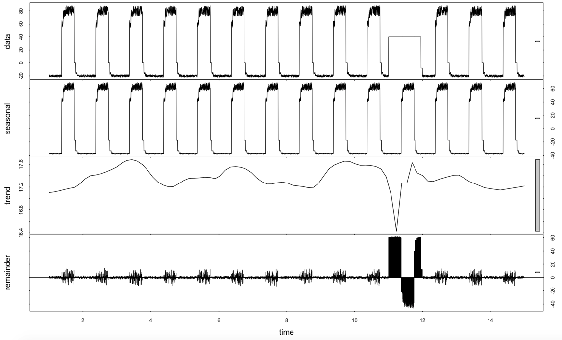
R版STL分解带噪音点数据的结果如下图:
data = read.csv("artificialWithAnomaly/art_daily_flatmiddle.csv")
View(data)
data_decomp <- stl(ts(data[[2]], frequency = 1440/5), s.window = "periodic", robust = TRUE)
plot(data_decomp)
statsmodels模块的时序分解的结果如下图:
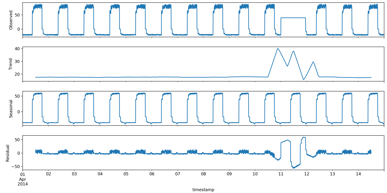
import statsmodels.api as sm
import matplotlib.pyplot as plt
import pandas as pd
from date_utils import get_gran, format_timestamp


dta = pd.read_csv('artificialWithAnomaly/art_daily_flatmiddle.csv',
                                   usecols=['timestamp', 'value'])
dta = format_timestamp(dta)
dta = dta.set_index('timestamp')
dta['value'] = dta['value'].apply(pd.to_numeric, errors='ignore')
dta.value.interpolate(inplace=True)
res = sm.tsa.seasonal_decompose(dta.value, freq=288)
res.plot()
plt.show()
2. 参考资料
[1] Cleveland, Robert B., William S. Cleveland, and Irma Terpenning. "STL: A seasonal-trend decomposition procedure based on loess." Journal of Official Statistics 6.1 (1990): 3.