1.
f=[-3,-1,0,0];
A=[2,-1,0,0];
b=[12];
Aeq=[3,3,1,0
    4,-4,0,1];
beq=[30,16];
lb=[0,0,0,0];
ub=[];
[x,y] = linprog(f,A,b,Aeq,beq,lb,ub)
Optimal solution found.
x =
6.999999999999999
3.000000000000000
0
0
y =
-23.999999999999996

library("Rglpk")
#a numeric vector representing the objective coefficients.
obj <- c(-2,-1,3,-5)
#a numeric vector or a (sparse) matrix of constraint coefficients.
mat <- matrix(c(1,2,1,2,3,0,4,-1,1,-1,1,1), nrow = 3)
#a character vector with the directions of the constraints.
dir <- c("<=", "<=", "<=")
#a numeric vector representing the right hand side of the constraints.
rhs <- c(6,12,4)
Rglpk_solve_LP(obj, mat, dir, rhs, max = FALSE)
$optimum
[1] -22.66667
$solution
[1] 0.000000 2.666667 0.000000 4.000000
2.
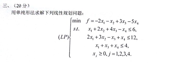
f=[-2,-1,3,-5];
A=[1,2,4,-1
    2,3,-1,1
    1,0,1,1];
b=[6,12,4];
Aeq=[];
beq=[];
lb=[0,0,0,0];
ub=[];
[x,y] = linprog(f,A,b,Aeq,beq,lb,ub)
Optimal solution found.
x =
0
2.666666666666667
0
4.000000000000001
y =
-22.666666666666671