MATLAB神经网络（2）之R练习

1. AMORE

1.1 newff

newff(n.neurons, learning.rate.global, momentum.global, error.criterium, Stao, hidden.layer, output.layer, method)

n.neurons：包含每层神经元的数值向量。第一个元素是输入神经元的数量，最后一个元素是输出神经元的数量，剩余的是隐含层神经元的数量；
learning.rate.global：每个神经元训练时的学习效率；
momentum.global：每个神经元的动量，仅几个训练算法需要该参数；
error.criterium：用于度量神经网络预测目标值接近程度的标准，可以使用以下几项：
"LMS"：Least Mean Squares

"LMLS"：Least Mean Logarithm Squared

"TAO"：TAO Error
Stao：当上一项为TAO时的Stao参数，对于其他的误差标准无用
hidden.layer：隐含层神经元的激活函数，可用："purelin"、"tansig"、"sigmoid"、"hardlim"、"custom"，其中"custom"表示需要用户自定义神经元的f0和f1元素；
output.layer：输出层神经元的激活函数；
method：优先选择的训练方法，包括：
"ADAPTgd": Adaptative gradient descend.（自适应的梯度下降方法）
"ADAPTgdwm": Adaptative gradient descend with momentum.（基于动量因子的自适应梯度下降方法）
"BATCHgd": BATCH gradient descend.（批量梯度下降方法）
"BATCHgdwm": BATCH gradient descend with momentum.（基于动量因子的批量梯度下降方法）

1.2 train

train(net, P, T, Pval=NULL, Tval=NULL, error.criterium="LMS", report=TRUE, n.shows, show.step, Stao=NA, prob=NULL, n.threads=0L)

net：要训练的神经网络；
P：训练集输入值；
T：训练集输出值；
Pval：验证集输入值；
Tval：验证集输出值；
error.criterium：度量拟合优劣程度的标准；
Stao：用于TAO算法的参数初始值；
report：逻辑值，是否打印训练过程信息；
n.shows：当上一项为TRUE时，打印的总次数；
show.step：训练过程一直进行到函数允许打印报告信息时经历的迭代次数；
prob：每一个样本应用到再抽样训练时的概率向量；
n.threads：用于BATCH*训练方法的线程数量，如果小于1，它将产生NumberProcessors-1个线程，其中NumberProcessors为处理器的个数，如果没有找到OpenMP库，该参数将被忽略。

1.3 example

library(AMORE)
# P is the input vector
P <- matrix(sample(seq(-1,1,length=1000), 1000, replace=FALSE), ncol=1) 
# The network will try to approximate the target P^2
target <- P^2                                   
# We create a feedforward network, with two hidden layers.
# The first hidden layer has three neurons and the second has two neurons.
# The hidden layers have got Tansig activation functions and the output layer is Purelin.
net <- newff(n.neurons=c(1,3,2,1), learning.rate.global=1e-2, momentum.global=0.5,
        error.criterium="LMS", Stao=NA, hidden.layer="tansig", 
        output.layer="purelin", method="ADAPTgdwm")
result <- train(net, P, target, error.criterium="LMS", report=TRUE, show.step=100, n.shows=5 )
P_test <- matrix(sample(seq(-1,1,length=1000), 100, replace=FALSE), ncol=1)
target_test <- P_test^2
y_test <- sim(result$net, P_test)
plot(P_test,y_test-target_test)

index.show: 1 LMS 0.0893172434474773
index.show: 2 LMS 0.0892277761187557
index.show: 3 LMS 0.000380711026069436
index.show: 4 LMS 0.000155618390342181
index.show: 5 LMS 9.53881309223154e-05

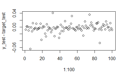
1.4 exercise

P <- matrix(rnorm(2000),ncol=2)
target <- apply(P^2,1,mean)
net <- newff(n.neurons=c(2,20,1),
             learning.rate.global=1e-2,
             momentum.global=0.5,
             error.criterium="LMS", 
             Stao=NA, 
             hidden.layer="tansig",
             output.layer="purelin", 
             method="ADAPTgdwm")
result <- train(net, P, target, 
                error.criterium="LMS", 
                report=TRUE, 
                show.step=100, 
                n.shows=10)
P_test <- matrix(rnorm(200),ncol=2) 
target_test <- apply(P_test^2,1,mean)
y_test <- sim(result$net, P_test)
plot(1:100,y_test-target_test)
(mean(abs(y_test-target_test)/target_test))

index.show: 1 LMS 0.00334168377394762
index.show: 2 LMS 0.00234274830312042
index.show: 3 LMS 0.00153074744985914
index.show: 4 LMS 0.00107702325684643
index.show: 5 LMS 0.000808644341077497
index.show: 6 LMS 0.000618371026226565
index.show: 7 LMS 0.000464896136767987
index.show: 8 LMS 0.000367196186841271
index.show: 9 LMS 0.00030261519286547
index.show: 10 LMS 0.000256892157194439
[1] 0.02934992

2. RSNNS

2.1 mlp

mlp(x, y, size = c(5), maxit = 100, initFunc = "Randomize_Weights", initFuncParams = c(-0.3, 0.3), learnFunc = "Std_Backpropagation", learnFuncParams = c(0.2, 0), updateFunc = "Topological_Order", updateFuncParams = c(0),
hiddenActFunc = "Act_Logistic", shufflePatterns = TRUE, linOut = FALSE, outputActFunc = if (linOut) "Act_Identity" else "Act_Logistic", inputsTest = NULL, targetsTest = NULL, pruneFunc = NULL, pruneFuncParams = NULL, ...)

x：一个矩阵，作为训练数据用于神经网络的输入；
y：对应的目标值；
size：隐含层单元的数量，默认为c(5)，当设置多个值时，表示有多个隐含层；
maxit：学习过程的最大迭代次数，默认为100；
initFunc：使用的初始化函数，默认为Randomize_Weights，即随机权重；
initFuncParams：用于初始化函数的参数，默认参数为c(-0.3,0.3)；
learnFunc：使用的学习函数，默认为Std_Backpropagation；
learnFuncParams：用于学习函数的参数，默认为c(0.2,0)；
updateFunc：使用的更新函数，默认为Topological_Order；
undateFuncParams：用于更新函数的参数，默认为c(0)；
hiddenActFunc：所有隐含层神经元的激活函数，默认为Act_Logistic；
shufflePatterns：是否将模式打乱，默认为TRUE；
linOut，设置输出神经元的激活函数，linear或者logistic，默认为FALSE；
inputsTest：一个矩阵，作为测试数据用于神经网络的输入，默认为NULL；
targetsTest：与测试输入对应的目标值，默认为NULL；
pruneFunc：使用的修剪函数，默认为NULL；
pruneFuncParams：用于修剪函数的函数，默认为NULL。

2.2 example

数据准备

library(RSNNS)
data(iris)

#shuffle the vector
iris <- iris[sample(1:nrow(iris),nrow(iris)),]

irisValues <- iris[,1:4]
irisTargets <- decodeClassLabels(iris[,5])
#irisTargets <- decodeClassLabels(iris[,5], valTrue=0.9, valFalse=0.1)

decodeClassLabels: This method decodes class labels from a numerical or levels vector to a binary matrix, i.e., it converts the input vector to a binary matrix.

> head(irisTargets)
     setosa versicolor virginica
[1,]      1          0         0
[2,]      0          1         0
[3,]      0          0         1
[4,]      1          0         0
[5,]      0          0         1
[6,]      0          0         1

抽样

iris <- splitForTrainingAndTest(irisValues, irisTargets, ratio=0.15)
iris <- normTrainingAndTestSet(iris)

splitForTrainingAndTest: Split the input and target values to a training and a test set. Test set is taken from the end of the data. If the data is to be shuffled, this should be done before calling this function.
normTrainingAndTestSet: Normalize training and test set as obtained by splitForTrainingAndTest in the following way: The inputsTrain member is normalized using normalizeData with the parameters given in type. The normalization parameters obtained during this normalization are then used to normalize the inputsTest member. if dontNormTargets is not set, then the targets are normalized in the same way. In classification problems, normalizing the targets normally makes no sense. For regression, normalizing also the targets is usually a good idea. The default is to not normalize targets values.

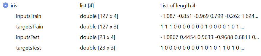
> attr(iris$inputsTrain,"normParams")$type
[1] "norm"
> attr(iris$inputsTest,"normParams")$type
[1] "norm"

训练&测试

model <- mlp(iris$inputsTrain, iris$targetsTrain, 
             size=5, 
             learnFuncParams=c(0.1),
             maxit=50, 
             inputsTest=iris$inputsTest,
             targetsTest=iris$targetsTest)

summary(model)

SNNS network definition file V1.4-3D
generated at Tue Feb 18 16:06:54 2020

network name : RSNNS_untitled
source files :
no. of units : 12（4+5+3=12个神经元）
no. of connections : 35（4×5+5×3=35权重）
no. of unit types : 0
no. of site types : 0

learning function : Std_Backpropagation
update function : Topological_Order

unit default section :

act | bias | st | subnet | layer | act func | out func
---------|----------|----|--------|-------|--------------|-------------
0.00000 | 0.00000 | i | 0 | 1 | Act_Logistic | Out_Identity
---------|----------|----|--------|-------|--------------|-------------

unit definition section :（给出偏置等参数）

no. | typeName | unitName | act | bias | st | position | act func | out func | sites
----|----------|-------------------|----------|----------|----|----------|--------------|----------|-------
1 | | Input_1 | 0.30243 | 0.27615 | i | 1,0,0 | Act_Identity | |
2 | | Input_2 | -0.55103 | 0.28670 | i | 2,0,0 | Act_Identity | |
3 | | Input_3 | 0.51752 | 0.05927 | i | 3,0,0 | Act_Identity | |
4 | | Input_4 | -0.00309 | 0.27664 | i | 4,0,0 | Act_Identity | |
5 | | Hidden_2_1 | 0.76338 | 1.91173 | h | 1,2,0 |||
6 | | Hidden_2_2 | 0.20872 | -2.48788 | h | 2,2,0 |||
7 | | Hidden_2_3 | 0.19751 | -0.35229 | h | 3,2,0 |||
8 | | Hidden_2_4 | 0.03343 | -1.45754 | h | 4,2,0 |||
9 | | Hidden_2_5 | 0.89784 | 0.82294 | h | 5,2,0 |||
10 | | Output_setosa | 0.05013 | -0.63914 | o | 1,4,0 |||
11 | | Output_versicolor | 0.82301 | -0.62233 | o | 2,4,0 |||
12 | | Output_virginica | 0.11542 | -1.02579 | o | 3,4,0 |||
----|----------|-------------------|----------|----------|----|----------|--------------|----------|-------

connection definition section :（给出权重矩阵）

target | site | source:weight
-------|------|---------------------------------------------------------------------------------------------------------------------
5 | | 4:-2.27555, 3:-1.59991, 2: 0.00019, 1: 0.26665
6 | | 4: 2.54355, 3: 1.83954, 2:-0.49918, 1:-0.21152
7 | | 4:-1.29117, 3:-0.90530, 2: 0.95187, 1:-0.20054
8 | | 4:-1.49130, 3:-1.54012, 2: 1.55497, 1:-0.85142
9 | | 4: 1.35965, 3: 1.07292, 2:-1.20123, 1: 0.45480
10 | | 9:-2.51547, 8: 2.26887, 7: 1.42713, 6:-2.24000, 5: 0.08607
11 | | 9: 1.31081, 8:-3.15358, 7:-1.09917, 6:-3.07740, 5: 2.55070
12 | | 9: 1.16730, 8:-2.03073, 7:-2.15568, 6: 2.90927, 5:-2.84570
-------|------|---------------------------------------------------------------------------------------------------------------------

> model

Class: mlp->rsnns
Number of inputs: 4
Number of outputs: 3
Maximal iterations: 50
Initialization function: Randomize_Weights
Initialization function parameters: -0.3 0.3
Learning function: Std_Backpropagation
Learning function parameters: 0.1
Update function:Topological_Order
Update function parameters: 0
Patterns are shuffled internally: TRUE
Compute error in every iteration: TRUE
Architecture Parameters:
$`size`
[1] 5

All members of model:
[1] "nInputs" "maxit"
[3] "initFunc" "initFuncParams"
[5] "learnFunc" "learnFuncParams"
[7] "updateFunc" "updateFuncParams"
[9] "shufflePatterns" "computeIterativeError"
[11] "snnsObject" "archParams"
[13] "IterativeFitError" "IterativeTestError"
[15] "fitted.values" "fittedTestValues"
[17] "nOutputs"

weightMatrix(model)
#extractNetInfo(model)

	Hidden_2_1	Hidden_2_2	Hidden_2_3	Hidden_2_4	Hidden_2_5	Output_setosa	Output_versicolor	Output_virginica
Input_1	0.2666532695	-0.2115191	-0.2005364	-0.8514175	0.4547978	0.00000000	0.000000	0.000000
Input_2	0.0001948424	-0.4991824	0.9518659	1.5549698	-1.2012329	0.00000000	0.000000	0.000000
Input_3	-1.5999110937	1.8395387	-0.9053020	-1.5401160	1.0729166	0.00000000	0.000000	0.000000
Input_4	-2.2755548954	2.5435514	-1.2911705	-1.4912956	1.3596520	0.00000000	0.000000	0.000000
Hidden_2_1	0.0000000000	0.0000000	0.0000000	0.0000000	0.0000000	0.08606748	2.550698	-2.845704
Hidden_2_2	0.0000000000	0.0000000	0.0000000	0.0000000	0.0000000	-2.24000168	-3.077400	2.909271
Hidden_2_3	0.0000000000	0.0000000	0.0000000	0.0000000	0.0000000	1.42712903	-1.099168	-2.155685
Hidden_2_4	0.0000000000	0.0000000	0.0000000	0.0000000	0.0000000	2.26887059	-3.153584	-2.030726
Hidden_2_5	0.0000000000	0.0000000	0.0000000	0.0000000	0.0000000	-2.51547217	1.310814	1.167299
Output_setosa	0.0000000000	0.0000000	0.0000000	0.0000000	0.0000000	0.00000000	0.000000	0.000000
Output_versicolor	0.0000000000	0.0000000	0.0000000	0.0000000	0.0000000	0.00000000	0.000000	0.000000
Output_virginica	0.0000000000	0.0000000	0.0000000	0.0000000	0.0000000	0.00000000	0.000000	0.000000

结果分析

绘出随迭代次数增加，误差平方和（SSE）的变化情况。

plotIterativeError(model)

散点为真实值和预测值的分布，黑色线为$y=x$，红色线为一次回归线。

predictions <- predict(model,iris$inputsTest)

plotRegressionError(predictions[,2], iris$targetsTest[,2])

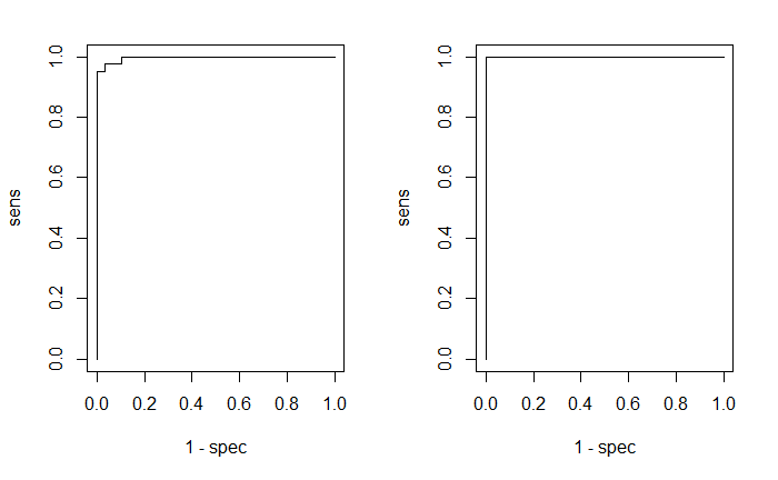
列出混淆矩阵，绘出EOC曲线。

> confusionMatrix(iris$targetsTrain,fitted.values(model))
       predictions
targets  1  2  3
      1 42  0  0
      2  0 38  2
      3  0  1 44
> confusionMatrix(iris$targetsTest,predictions)
       predictions
targets 1 2 3
      1 8 0 0
      2 0 9 1
      3 0 0 5

par(mfrow=c(1,2))
plotROC(fitted.values(model)[,2], iris$targetsTrain[,2])
plotROC(predictions[,2], iris$targetsTest[,2])

给出更严格的检验，若3项中1项大于0.6，其余两项小于0.4，则将其归为该项，否则标0，视为无法判定。

> confusionMatrix(iris$targetsTrain, 
+                 encodeClassLabels(fitted.values(model),
+                                   method="402040", l=0.4, h=0.6))
       predictions
targets  0  1  2  3
      1  0 42  0  0
      2  4  0 36  0
      3  3  0  0 42