1.数据准备
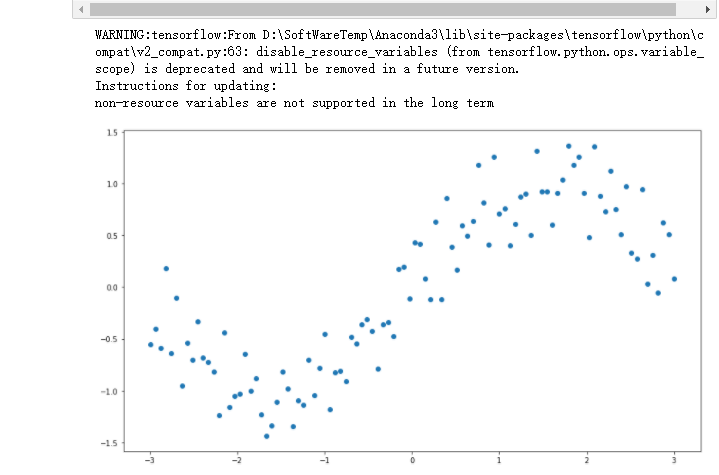
%matplotlib inline
import numpy as np
#import tensorflow as tf#
#引入tensorflow 并保证 placeholder 可以使用
import tensorflow.compat.v1 as tf
tf.disable_v2_behavior()
import matplotlib.pyplot as plt
## 设置figure_size尺寸
plt.rcParams["figure.figsize"] = (14,8)

n_observations = 100
#创建等差数列 -3到 3 100个
xs = np.linspace(-3, 3, n_observations)
#从一个均匀分布[low,high)中随机采样,注意定义域是左闭右开  numpy.random.uniform(low,high,size)
ys = np.sin(xs) + np.random.uniform(-0.5, 0.5, n_observations)
#绘制散点图 (x,y)平面的位置
plt.scatter(xs, ys)
plt.show()
2.准备好placeholder
# 定义参数的数据类型 数据形状(一般为一维)名称
X = tf.placeholder(tf.float32, name='X')
Y = tf.placeholder(tf.float32, name='Y')
# 设置参数为全局变量
global X
global Y
global W
3.初始化参数/权重
# tf.Variable(initializer,name) 初始化参数 和 自定义的变量名称
#tf.random_normal()函数用于从“服从指定正态分布的序列”中随机取出指定个数的值
W = tf.Variable(tf.random.normal([1]), name='weight')
b = tf.Variable(tf.random.normal([1]), name='bias')
4.计算预测结果
#预测值 tf.multiply()两个矩阵中对应元素各自相乘 tf.add() 将参数相加
Y_pred = tf.add(tf.multiply(X, W), b)
5.计算损失函数值
#损失函数  对a里的每一个元素求平方
loss = tf.square(Y - Y_pred, name='loss')
6.初始化optimizer
#学习率
learning_rate = 0.01
#optimizer = tf.train.GradientDescentOptimizer(learning_rate).minimize(loss)
# 实现梯度下降和会话流程
optimizer = tf.train.GradientDescentOptimizer(learning_rate).minimize(loss)
7.指定迭代次数,并在session里执行graph
n_samples = xs.shape[0]
with tf.Session() as sess:
    # 记得初始化所有变量
    sess.run(tf.global_variables_initializer())

    writer = tf.summary.FileWriter('./graphs/linear_reg', sess.graph)

    # 训练模型
    for i in range(50):
        total_loss = 0
        for x, y in zip(xs, ys):
            # 通过feed_dic把数据灌进去
            _, l = sess.run([optimizer, loss], feed_dict={X: x, Y:y})
            total_loss += l
        if i%5 ==0:
            print('Epoch {0}: {1}'.format(i, total_loss/n_samples))

    # 关闭writer
    writer.close()

    # 取出w和b的值
    W, b = sess.run([W, b])

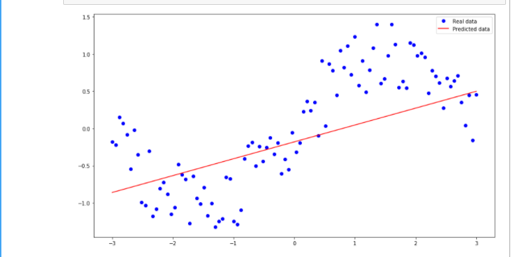
# 输出W b 的值
print(W,b)
print("W:"+str(W[0]))
print("b:"+str(b[0]))

#设置散点图的图例
plt.plot(xs, ys, 'bo', label='Real data')
plt.plot(xs, xs * W + b, 'r', label='Predicted data')
#给图像加上图例
plt.legend()
plt.show()