▶ 使用线性回归来为散点作分类
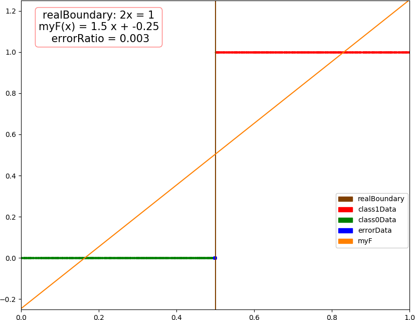
● 普通线性回归,代码
  1 import numpy as np
  2 import matplotlib.pyplot as plt
  3 from mpl_toolkits.mplot3d import Axes3D
  4 from mpl_toolkits.mplot3d.art3d import Poly3DCollection
  5 from matplotlib.patches import Rectangle
  6
  7 dataSize = 10000
  8 trainRatio = 0.3
  9 colors = [[0.5,0.25,0],[1,0,0],[0,0.5,0],[0,0,1],[1,0.5,0]] # 棕红绿蓝橙
 10 trans = 0.5
 11
 12 def dataSplit(data, part):                                  # 将数据集分割为训练集和测试集
 13     return data[0:part,:],data[part:,:]
 14
 15 def mySign(x):                                              # 区分 np.sign()
 16     return (1 + np.sign(x))/2
 17
 18 def function(x,para):                                       # 连续回归函数
 19     return np.sum(x * para[0]) + para[1]
 20
 21 def judge(x, para):                                         # 分类函数,由乘加部分和阈值部分组成
 22     return mySign(function(x, para) - 0.5)
 23
 24 def createData(dim, len):                                   # 生成测试数据
 25     np.random.seed(103)
 26     output=np.zeros([len,dim+1])
 27     for i in range(dim):
 28         output[:,i] = np.random.rand(len)
 29     output[:,dim] = list(map(lambda x : int(x > 0.5), (3 - 2 * dim)*output[:,0] + 2 * np.sum(output[:,1:dim], 1)))
 30     #print(output, "
", np.sum(output[:,-1])/len)
 31     return output
 32
 33 def linearRegression(data):                                 # 线性回归
 34     len,dim = np.shape(data)
 35     dim -= 1
 36     if(dim) == 1:                                           # 一元单独出来,其实可以合并到下面的 else 中
 37         sumX = np.sum(data[:,0])
 38         sumY = np.sum(data[:,1])
 39         sumXY = np.sum([x*y for x,y in data])
 40         sumXX = np.sum([x*x for x in data[:,0]])
 41         w = (sumXY * len - sumX * sumY) / (sumXX * len - sumX * sumX)
 42         b = (sumY - w * sumX) / len
 43         return ([w] , b)
 44     else:                                                   # 二元及以上,暂不考虑降秩的问题
 45         dataE = np.concatenate((data[:,:-1], np.ones(len)[:,np.newaxis]), axis = 1)
 46         w = np.matmul(np.matmul(np.linalg.inv(np.matmul(dataE.T, dataE)),dataE.T),data[:,-1]) # w = (X^T * X)^(-1) * X^T * y
 47         return (w[:-1],w[-1])
 48
 49 def test(dim):                                              # 测试函数
 50     allData = createData(dim, dataSize)
 51     trainData, testData = dataSplit(allData, int(dataSize * trainRatio))
 52
 53     para = linearRegression(trainData)
 54
 55     myResult = [ judge(i[0:dim], para) for i in testData ]
 56     errorRatio = np.sum((np.array(myResult) - testData[:,-1].astype(int))**2) / (dataSize*(1-trainRatio))
 57     print("dim = "+ str(dim) + ", errorRatio = " + str(round(errorRatio,4)))
 58     if dim >= 4:                                            # 4维以上不画图,只输出测试错误率
 59         return
 60
 61     errorP = []                                             # 画图部分,测试数据集分为错误类,1 类和 0 类
 62     class1 = []
 63     class0 = []
 64     for i in range(np.shape(testData)[0]):
 65         if myResult[i] != testData[i,-1]:
 66             errorP.append(testData[i])
 67         elif myResult[i] == 1:
 68             class1.append(testData[i])
 69         else:
 70             class0.append(testData[i])
 71     errorP = np.array(errorP)
 72     class1 = np.array(class1)
 73     class0 = np.array(class0)
 74
 75     fig = plt.figure(figsize=(10, 8))
 76
 77     if dim == 1:
 78         plt.xlim(0.0,1.0)
 79         plt.ylim(-0.25,1.25)
 80         plt.plot([0.5, 0.5], [-0.5, 1.25], color = colors[0],label = "realBoundary")
 81         plt.plot([0, 1], [ function(i, para) for i in [0,1] ],color = colors[4], label = "myF")
 82         plt.scatter(class1[:,0], class1[:,1],color = colors[1], s = 2,label = "class1Data")
 83         plt.scatter(class0[:,0], class0[:,1],color = colors[2], s = 2,label = "class0Data")
 84         if len(errorP) != 0:
 85             plt.scatter(errorP[:,0], errorP[:,1],color = colors[3], s = 16,label = "errorData")
 86         plt.text(0.2, 1.12, "realBoundary: 2x = 1
myF(x) = " + str(round(para[0][0],2)) + " x + " + str(round(para[1],2)) + "
 errorRatio = " + str(round(errorRatio,4)),
 87             size=15, ha="center", va="center", bbox=dict(boxstyle="round", ec=(1., 0.5, 0.5), fc=(1., 1., 1.)))
 88         R = [Rectangle((0,0),0,0, color = colors[k]) for k in range(5)]
 89         plt.legend(R, ["realBoundary", "class1Data", "class0Data", "errorData", "myF"], loc=[0.81, 0.2], ncol=1, numpoints=1, framealpha = 1)
 90
 91     if dim == 2:
 92         plt.xlim(0.0,1.0)
 93         plt.ylim(0.0,1.0)
 94         plt.plot([0,1], [0.25,0.75], color = colors[0],label = "realBoundary")
 95         xx = np.arange(0, 1 + 0.1, 0.1)
 96         X,Y = np.meshgrid(xx, xx)
 97         contour = plt.contour(X, Y, [ [ function((X[i,j],Y[i,j]), para) for j in range(11)] for i in range(11) ])
 98         plt.clabel(contour, fontsize = 10,colors='k')
 99         plt.scatter(class1[:,0], class1[:,1],color = colors[1], s = 2,label = "class1Data")
100         plt.scatter(class0[:,0], class0[:,1],color = colors[2], s = 2,label = "class0Data")
101         if len(errorP) != 0:
102             plt.scatter(errorP[:,0], errorP[:,1],color = colors[3], s = 8,label = "errorData")
103         plt.text(0.75, 0.92, "realBoundary: -x + 2y = 1
myF(x,y) = " + str(round(para[0][0],2)) + " x + " + str(round(para[0][1],2)) + " y + " + str(round(para[1],2)) + "
 errorRatio = " + str(round(errorRatio,4)),
104             size = 15, ha="center", va="center", bbox=dict(boxstyle="round", ec=(1., 0.5, 0.5), fc=(1., 1., 1.)))
105         R = [Rectangle((0,0),0,0, color = colors[k]) for k in range(4)]
106         plt.legend(R, ["realBoundary", "class1Data", "class0Data", "errorData"], loc=[0.81, 0.2], ncol=1, numpoints=1, framealpha = 1)
107
108     if dim == 3:
109         ax = Axes3D(fig)
110         ax.set_xlim3d(0.0, 1.0)
111         ax.set_ylim3d(0.0, 1.0)
112         ax.set_zlim3d(0.0, 1.0)
113         ax.set_xlabel('X', fontdict={'size': 15, 'color': 'k'})
114         ax.set_ylabel('Y', fontdict={'size': 15, 'color': 'k'})
115         ax.set_zlabel('W', fontdict={'size': 15, 'color': 'k'})
116         v = [(0, 0, 0.25), (0, 0.25, 0), (0.5, 1, 0), (1, 1, 0.75), (1, 0.75, 1), (0.5, 0, 1)]
117         f = [[0,1,2,3,4,5]]
118         poly3d = [[v[i] for i in j] for j in f]
119         ax.add_collection3d(Poly3DCollection(poly3d, edgecolor = 'k', facecolors = colors[0]+[trans], linewidths=1))
120         ax.scatter(class1[:,0], class1[:,1],class1[:,2], color = colors[1], s = 2, label = "class1")
121         ax.scatter(class0[:,0], class0[:,1],class0[:,2], color = colors[2], s = 2, label = "class0")
122         if len(errorP) != 0:
123             ax.scatter(errorP[:,0], errorP[:,1],errorP[:,2], color = colors[3], s = 8, label = "errorData")
124         ax.text3D(0.8, 1, 1.15, "realBoundary: -3x + 2y +2z = 1
myF(x,y,z) = " + str(round(para[0][0],2)) + " x + " +
125             str(round(para[0][1],2)) + " y + " + str(round(para[0][2],2)) + " z + " + str(round(para[1],2)) + "
 errorRatio = " + str(round(errorRatio,4)),
126             size = 12, ha="center", va="center", bbox=dict(boxstyle="round", ec=(1, 0.5, 0.5), fc=(1, 1, 1)))
127         R = [Rectangle((0,0),0,0, color = colors[k]) for k in range(4)]
128         plt.legend(R, ["realBoundary", "class1Data", "class0Data", "errorData"], loc=[0.83, 0.1], ncol=1, numpoints=1, framealpha = 1)
129
130     fig.savefig("R:\dim" + str(dim) + ".png")
131     plt.close()
132
133 if __name__ == '__main__':
134     test(1)
135     test(2)
136     test(3)
137     test(4)
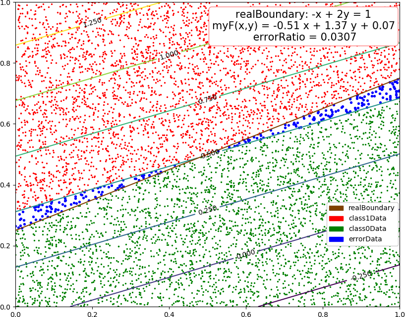
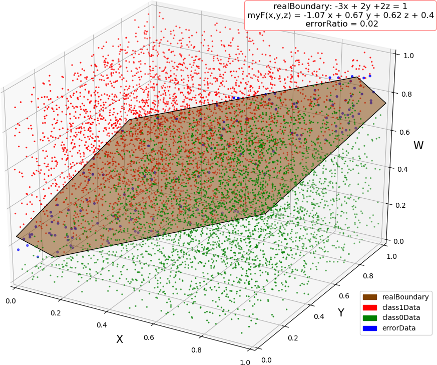
● 输出结果
dim = 1, errorRatio = 0.003
dim = 2, errorRatio = 0.0307
dim = 3, errorRatio = 0.02
dim = 4, errorRatio = 0.0349
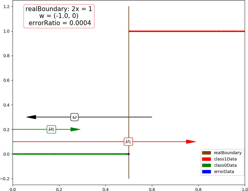
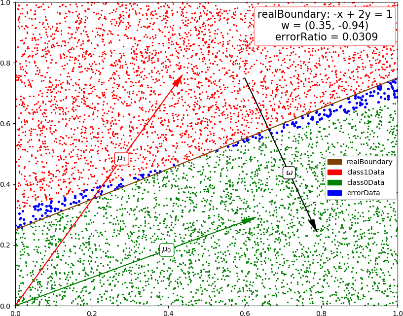
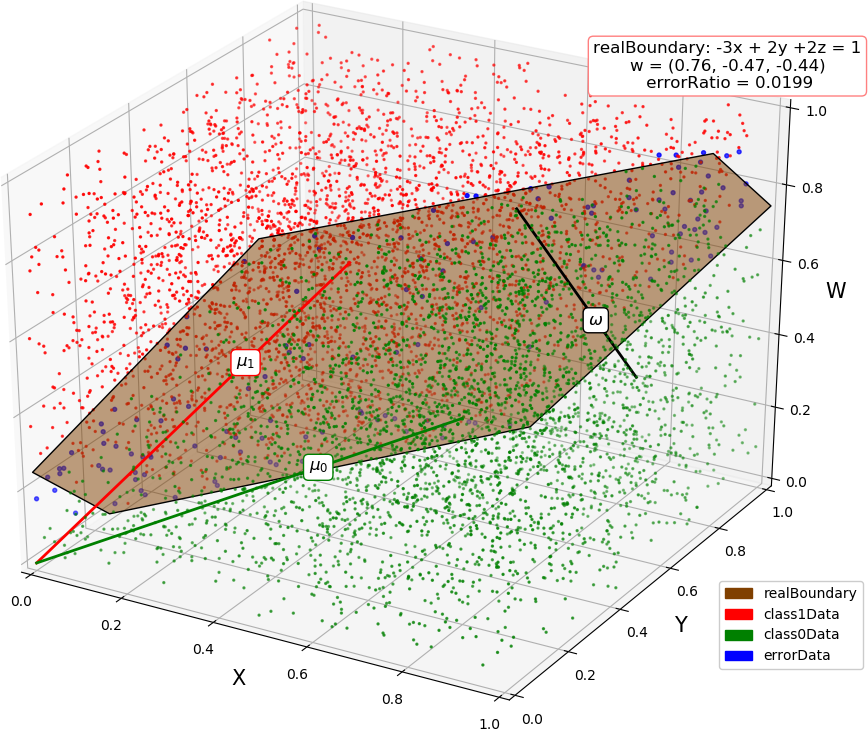
● LDA法,代码
  1 import numpy as np
  2 import matplotlib.pyplot as plt
  3 from mpl_toolkits.mplot3d import Axes3D
  4 from mpl_toolkits.mplot3d.art3d import Poly3DCollection
  5 from matplotlib.patches import Rectangle
  6
  7 dataSize = 10000
  8 trainRatio = 0.3
  9 colors = [[0.5,0.25,0],[1,0,0],[0,0.5,0],[0,0,1],[1,0.5,0],[0,0,0]] # 棕红绿蓝橙黑
 10 trans = 0.5
 11
 12 def dataSplit(data, part):                                  # 将数据集分割为训练集和测试集
 13     return data[0:part,:],data[part:,:]
 14
 15 def dot(x, w):                                              # 内积,返回标量
 16     return np.sum(x * w)
 17
 18 def judge(x, w, mu1pro, mu0pro):                            # 分类函数直接用欧氏距离
 19     return int(2 * dot(mu0pro - mu1pro, w * dot(x, w))< (dot(mu0pro, mu0pro) - dot(mu1pro, mu1pro)))
 20
 21 def createData(dim, len):                                   # 生成测试数据
 22     np.random.seed(103)
 23     output = np.zeros([len,dim+1])
 24     for i in range(dim):
 25         output[:,i] = np.random.rand(len)
 26     output[:,dim] = list(map(lambda x : int(x > 0.5), (3 - 2 * dim)*output[:,0] + 2 * np.sum(output[:,1:dim], 1)))
 27     #print(output, "
", np.sum(output[:,-1])/len)
 28     return output
 29
 30 def linearDiscriminantAnalysis(data):                       # LDA 法
 31     dim = np.shape(data)[1] - 1
 32     class1 = []
 33     class0 = []
 34     for line in data:
 35         if line[-1] > 0.5:
 36             class1.append(line)
 37         else:
 38             class0.append(line)
 39     class1 = np.array(class1)
 40     class0 = np.array(class0)
 41     mu1 = np.sum(class1[:,0:dim],0) / np.shape(class1)[0]
 42     mu0 = np.sum(class0[:,0:dim],0) / np.shape(class0)[0]
 43     temp1 = class1[:,0:dim] - mu1
 44     temp0 = class0[:,0:dim] - mu0
 45     w = np.matmul(np.linalg.inv(np.matmul(temp1.T,temp1) + np.matmul(temp0.T,temp0)),mu0 - mu1) # w = Sw^(-1) * (mu0 - m1)
 46     return (w / np.sqrt(dot(w, w)), mu1, mu0)
 47
 48 def test(dim):                                              # 测试函数
 49     allData = createData(dim, dataSize)
 50     trainData, testData = dataSplit(allData, int(dataSize * trainRatio))
 51
 52     para = linearDiscriminantAnalysis(trainData)
 53     mu1pro = para[0] * dot(para[1], para[0])
 54     mu0pro = para[0] * dot(para[2], para[0])
 55     myResult = [ judge(i[0:dim], para[0], mu1pro, mu0pro) for i in testData ]
 56     errorRatio = np.sum((np.array(myResult) - testData[:,-1].astype(int))**2) / (dataSize*(1-trainRatio))
 57     print("dim = "+ str(dim) + ", errorRatio = " + str(round(errorRatio,4)))
 58     if dim >= 4:                                            # 4维以上不画图,只输出测试错误率
 59         return
 60
 61     errorP = []                                             # 画图部分,测试数据集分为错误类,1 类和 0 类
 62     class1 = []
 63     class0 = []
 64     for i in range(np.shape(testData)[0]):
 65         if myResult[i] != testData[i,-1]:
 66             errorP.append(testData[i])
 67         elif myResult[i] == 1:
 68             class1.append(testData[i])
 69         else:
 70             class0.append(testData[i])
 71     errorP = np.array(errorP)
 72     class1 = np.array(class1)
 73     class0 = np.array(class0)
 74
 75     fig = plt.figure(figsize=(10, 8))
 76
 77     if dim == 1:
 78         plt.xlim(0.0,1.0)
 79         plt.ylim(-0.25,1.25)
 80         plt.plot([0.5, 0.5], [-0.2, 1.2], color = colors[0],label = "realBoundary")
 81         plt.arrow(0.6, 0.3, para[0][0]/2, 0, head_width=0.03, head_length=0.04, fc=colors[5], ec=colors[5])
 82         plt.arrow(0, 0.1, para[1][0], 0, head_width=0.03, head_length=0.04, fc=colors[1], ec=colors[1])
 83         plt.arrow(0, 0.2, para[2][0], 0, head_width=0.03, head_length=0.04, fc=colors[2], ec=colors[2])
 84         plt.scatter(class1[:,0], class1[:,1],color = colors[1], s = 2,label = "class1Data")
 85         plt.scatter(class0[:,0], class0[:,1],color = colors[2], s = 2,label = "class0Data")
 86         if len(errorP) != 0:
 87             plt.scatter(errorP[:,0], errorP[:,1],color = colors[3], s = 16,label = "errorData")
 88         plt.text(0.2, 1.12, "realBoundary: 2x = 1
w = (" + str(round(para[0][0],2)) + ", 0)
 errorRatio = " + str(round(errorRatio,4)),
 89             size=15, ha="center", va="center", bbox=dict(boxstyle="round", ec=(1., 0.5, 0.5), fc=(1., 1., 1.)))
 90         plt.text(0.6 + para[0][0]/3,0.3, "$omega$", size = 12, ha="center", va="center", bbox=dict(boxstyle="round", ec=colors[5], fc=(1., 1., 1.)))
 91         plt.text(para[1][0]*2/3,0.1, "$mu_{1}$", size = 12, ha="center", va="center", bbox=dict(boxstyle="round", ec=colors[1], fc=(1., 1., 1.)))
 92         plt.text(para[2][0]*2/3,0.2, "$mu_{0}$", size = 12, ha="center", va="center", bbox=dict(boxstyle="round", ec=colors[2], fc=(1., 1., 1.)))
 93         R = [Rectangle((0,0),0,0, color = colors[k]) for k in range(4)]
 94         plt.legend(R, ["realBoundary", "class1Data", "class0Data", "errorData"], loc=[0.81, 0.05], ncol=1, numpoints=1, framealpha = 1)
 95
 96     if dim == 2:
 97         plt.xlim(0.0,1.0)
 98         plt.ylim(0.0,1.0)
 99         plt.plot([0,1], [0.25,0.75], color = colors[0],label = "realBoundary")
100
101         plt.arrow(0.6, 0.75, para[0][0]/2, para[0][1]/2, head_width=0.015, head_length=0.04, fc=colors[5], ec=colors[5])
102         plt.arrow(0, 0, para[1][0], para[1][1], head_width=0.015, head_length=0.04, fc=colors[1], ec=colors[1])
103         plt.arrow(0, 0, para[2][0], para[2][1], head_width=0.015, head_length=0.04, fc=colors[2], ec=colors[2])
104         plt.scatter(class1[:,0], class1[:,1],color = colors[1], s = 2,label = "class1Data")
105         plt.scatter(class0[:,0], class0[:,1],color = colors[2], s = 2,label = "class0Data")
106         if len(errorP) != 0:
107             plt.scatter(errorP[:,0], errorP[:,1],color = colors[3], s = 8,label = "errorData")
108         plt.text(0.81, 0.92, "realBoundary: -x + 2y = 1
w = (" + str(round(para[0][0],2)) + ", " + str(round(para[0][1],2)) + ")
 errorRatio = " + str(round(errorRatio,4)),
109             size = 15, ha="center", va="center", bbox=dict(boxstyle="round", ec=(1., 0.5, 0.5), fc=(1., 1., 1.)))
110         plt.text(0.6 + para[0][0]/3,0.75+para[0][1]/3, "$omega$", size = 12, ha="center", va="center", bbox=dict(boxstyle="round", ec=colors[5], fc=(1., 1., 1.)))
111         plt.text(para[1][0]*2/3,para[1][1]*2/3, "$mu_{1}$", size = 12, ha="center", va="center", bbox=dict(boxstyle="round", ec=colors[1], fc=(1., 1., 1.)))
112         plt.text(para[2][0]*2/3,para[2][1]*2/3, "$mu_{0}$", size = 12, ha="center", va="center", bbox=dict(boxstyle="round", ec=colors[2], fc=(1., 1., 1.)))
113
114         R = [Rectangle((0,0),0,0, color = colors[k]) for k in range(4)]
115         plt.legend(R, ["realBoundary", "class1Data", "class0Data", "errorData"], loc=[0.81, 0.35], ncol=1, numpoints=1, framealpha = 1)
116
117     if dim == 3:
118         ax = Axes3D(fig)
119         ax.set_xlim3d(0.0, 1.0)
120         ax.set_ylim3d(0.0, 1.0)
121         ax.set_zlim3d(0.0, 1.0)
122         ax.set_xlabel('X', fontdict={'size': 15, 'color': 'k'})
123         ax.set_ylabel('Y', fontdict={'size': 15, 'color': 'k'})
124         ax.set_zlabel('W', fontdict={'size': 15, 'color': 'k'})
125         v = [(0, 0, 0.25), (0, 0.25, 0), (0.5, 1, 0), (1, 1, 0.75), (1, 0.75, 1), (0.5, 0, 1)]
126         f = [[0,1,2,3,4,5]]
127         poly3d = [[v[i] for i in j] for j in f]
128         ax.add_collection3d(Poly3DCollection(poly3d, edgecolor = 'k', facecolors = colors[0]+[trans], linewidths=1))
129         ax.plot([0.6, 0.6 + para[0][0]/2],[0.75, 0.75 + para[0][1]/2],[0.75, 0.75 + para[0][2]/2], color = colors[5], linewidth = 2)    # 手工线段代替箭头
130         ax.plot([0,para[1][0]],[0,para[1][1]],[0,para[1][2]], color = colors[1], linewidth = 2)
131         ax.plot([0,para[2][0]],[0,para[2][1]],[0,para[2][2]], color = colors[2], linewidth = 2)
132         ax.scatter(class1[:,0], class1[:,1],class1[:,2], color = colors[1], s = 2, label = "class1")
133         ax.scatter(class0[:,0], class0[:,1],class0[:,2], color = colors[2], s = 2, label = "class0")
134         if len(errorP) != 0:
135             ax.scatter(errorP[:,0], errorP[:,1],errorP[:,2], color = colors[3], s = 8, label = "errorData")
136         ax.text3D(0.85, 1.1, 1.03, "realBoundary: -3x + 2y +2z = 1
w = (" + str(round(para[0][0],2)) + ", " + str(round(para[0][1],2)) + ", " + str(round(para[0][2],2)) +")
 errorRatio = " + str(round(errorRatio,4)),
137             size = 12, ha="center", va="center", bbox=dict(boxstyle="round", ec=(1, 0.5, 0.5), fc=(1, 1, 1)))
138         ax.text3D(0.6 + para[0][0]/3,0.75+para[0][1]/3, 0.75+para[0][2]/3, "$omega$", size = 12, ha="center", va="center", bbox=dict(boxstyle="round", ec=colors[5], fc=(1., 1., 1.)))
139         ax.text3D(para[1][0]*2/3,para[1][1]*2/3, para[1][2]*2/3, "$mu_{1}$", size = 12, ha="center", va="center", bbox=dict(boxstyle="round", ec=colors[1], fc=(1., 1., 1.)))
140         ax.text3D(para[2][0]*2/3,para[2][1]*2/3, para[2][2]*2/3, "$mu_{0}$", size = 12, ha="center", va="center", bbox=dict(boxstyle="round", ec=colors[2], fc=(1., 1., 1.)))
141
142         R = [Rectangle((0,0),0,0, color = colors[k]) for k in range(4)]
143         plt.legend(R, ["realBoundary", "class1Data", "class0Data", "errorData"], loc=[0.83, 0.1], ncol=1, numpoints=1, framealpha = 1)
144
145     fig.savefig("R:\dim" + str(dim) + ".png")
146     plt.close()
147
148 if __name__ == '__main__':
149     test(1)
150     test(2)
151     test(3)
152     test(4)
● 输出结果
dim = 1, errorRatio = 0.0004
dim = 2, errorRatio = 0.0309
dim = 3, errorRatio = 0.0199
dim = 4, errorRatio = 0.0349