看到有不少人挺推崇:An overview of gradient descent optimization algorithms;特此放到最上面,大家有机会可以阅读一下;
本文内容主要来源于Coursera吴恩达《优化深度神经网络》课程,另外一些不同优化算法之间的比较也会出现在其中,具体来源不再单独说明,会在文末给出全部的参考文献;
本主要主要介绍的优化算法有:
- Mini-batch梯度下降(Mini-batch gradient descent)
- 指数加权平均(Exponentially weighted averages)
- Momentum梯度下降法
- RMSprop算法
- Adam算法
其实就是对梯度下降的优化算法,每一种优化算法会介绍其:基本原理、TensorFlow中的使用、不同优化算法的优缺点总结;在最后会介绍调整学习率衰减的方式以及局部最优问题;
1. Mini-batch gradient descent
如果样本数量不是过于庞大,一般使用batch的方式进行计算,即将整个样本集投入到深度神经网络进行梯度下降;而一般实际应用中,样本集的数量将会很大,如达到百万数量级,这种情况下如果继续使用batch的方式,训练的速度往往会很慢;
因此,假如每次只对整个样本集中的部分样本执行梯度下降,这就有了Mini-batch gradient descent。
1.1 算法原理
整个样本集\(X=[x^1, x^2, \cdots, x^m] \in R^{n \times m}\);\(Y=[y^1, y^2, \cdots, y^m] \in R^{1 \times m}\);
假设:
\(m=5000000\);每一个mini-batch含有1000个样本,即\(X^{\{t\}} \in R^{n \times 1000},Y^{\{t\}} \in R^{1 \times 1000}, t=1, 2, \cdots, 5000\);
\(x^i\)表示第\(i\)个样本;\(Z^{[l]}\)表示网络第\(l\)层网络的线性输出;\(X^{\{t\}}, Y^{\{t\}}\)表示第\(t\)组mini-batch;
即在每一个mini-batch上执行梯度下降,伪代码如下:
# 一个epoch
for t = 1, ..., T{
    Forward Propagation
    Compute Cost Function
    Backward Propagation
}
其中,每一步详解:
(1)Forward Propagation
第一层网络非线性输出:
第\(l\)层网络非线性输出:
(2)Compute Cost Function
计算代价函数:
(3)Backward Propagation
更新权重和偏置:
经过T次for循环后,表示已经在整个样本集上训练了一次,即一个epoch;可以执行多个epoch;
1.2 进一步理解Mini-batch gradient descent
对与Batch Gradient Descent来说,一个epoch只进行了一次梯度下降;而对于Mini-batch Gradient Decent来说,一个epoch进行T次梯度下降;
1.2.1 Cost function
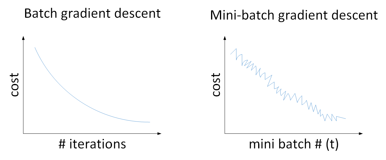
(1)左图表示一般神经网络中,使用Batch Gradient Descent,随着在整个样本集上迭代次数的增加,cost在不断的减小;
(2)右图表示使用Mini-batch Gradient Descent,随着在不同的mini-batch上进行训练,cost整体趋势处于下降,但由于受到噪声的影响,会出现震荡;
(3)Mini-batch Gradient Descent中cost出现震荡的原因时:不同的mini-batch之间是存在差异的,可能其中某些mini-batch是好的子集,而某些子集中存在噪声,因此cost会出现震荡的情况;
1.2.2 如何选择batch size
总共有三种选择方式:(1)batch_size=m;(2)batch_size=1;(3)batch_size介于1和m之间;
(1)Batch Gradient Descent(batch_size = m)
当batch_size=m,就成了Batch Gradient Descent,只有包含一个子集,就是整个数据集;即\((X^{\{1\}}, Y^{\{1\}})=(X,Y)\);
(2)Stochastic Gradient Descent(batch_size=1)
当batch_size=m,就成了Stochastic Gradient Descent,共包含m个子集,每个样本作为一个子集,即\((X^{\{1\}}, Y^{\{1\}})=(x^i,y^i)\);
(3)Mini-batch gradient descent(batch_size介于1和m之间)
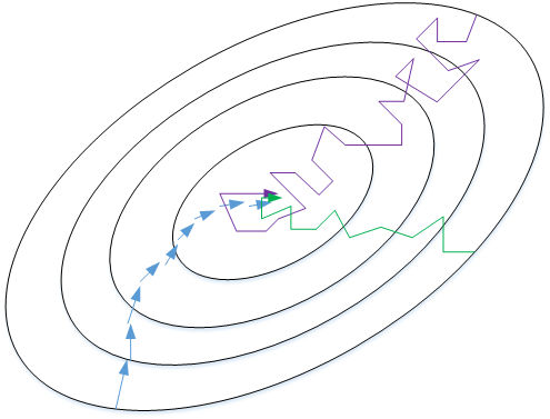
上图表示三者之间梯度下降曲线:
a. 蓝色表示Batch Gradient Descent,会比较平稳的接近全局最小值;由于使用了全部数据集,每次前进的速度会比较慢;
b. 紫色表示Stochastic Gradient Descent,每次前进速度很快;但由于每次只使用了一个样本,会出现较大的震荡;而且,不会收敛到最小值,最终会在最小值附近来回波动
c. 绿色表示Mini-batch gradient descent,每次前进速度较快,且震荡较小,基本能够接近最小值;如果出现在最小值附近波动,可以减小学习率;
| 算法 | Stochastic Gradient Descent | Mini-batch gradient descent | Batch Gradient Descent |
|---|---|---|---|
| 优点 | 适用于单个样本; | (1)能够快速学习;(2)向量化加速;(3)未在整个训练集上训练完,就可以执行后续工作; | |
| 缺点 | (1)丢失了向量化带来的加速;(2)效率低; | 单次迭代时间太长; |
如何为Mini-batch gradient descent选择batch size?
- 64-512,2的n次方,提高运算速度;
- \(X^{\{t\}}, Y^{\{t\}}\)符合GPU、CPU内存;
1.3 TensorFlow中的梯度下降
1.3.1 构建optimizer
optimizer = tf.train.GradientDescentOptimizer(leraning_rate)
train = optimizer.minimize(loss)
1.3.2 tf.train.GradientDescentOptimizer()
tf.train.GradientDescentOptimizer.__init__(self,
                                           learning_rate,
                                           use_locking=False,
                                           name="GradientDescent"):
Args:
	learning_rate: A Tensor or a floating point value.  The learning rate to use.  # 学习率
	use_locking: If True use locks for update operations.  #
	name: Optional name prefix for the operations created when applying gradients. Defaults to "GradientDescent".
1.3.3 TensorFlow中的使用
#coding=utf-8
import tensorflow as tf

# Model parameters
W = tf.Variable([.3], dtype=tf.float32)
b = tf.Variable([-.3], dtype=tf.float32)
# Model input and output
x = tf.placeholder(tf.float32)
y_pred = W * x + b
y = tf.placeholder(tf.float32)

# loss
loss = tf.reduce_sum(tf.square(y_pred - y))  # sum of the squares
# optimizer
optimizer = tf.train.GradientDescentOptimizer(0.01)
train = optimizer.minimize(loss)

# training data
x_train = [1, 2, 3, 4]
y_train = [0, -1, -2, -3]
# training loop
init = tf.global_variables_initializer()
sess = tf.Session()
sess.run(init)  # reset values to wrong
for i in range(1000):
    sess.run(train, {x: x_train, y: y_train})

# evaluate training accuracy
curr_W, curr_b, curr_loss = sess.run([W, b, loss], {x: x_train, y: y_train})
print("W: %s b: %s loss: %s" % (curr_W, curr_b, curr_loss))
2. Exponentially weighted averages
指数加权平均(Exponentially weighted averages)是除梯度下降算法之外其他优化算法中重要的概念,因此,这里先介绍其概念。
2.1 伦敦天气温度
这里不再介绍如何引入指数加权平均的,具体参考:网易云课堂-吴恩达《优化深度神经网络》-第二周或红色石头Will-吴恩达《优化深度神经网络》课程笔记;
假设:\(V_0 = 0\);
其中,\(\theta_t\)表示第\(t\)天的温度;\(V_t\)表示通过移动平均的方法对每天气温进行平滑处理后结果;
\(\beta\)值决定了指数加权平均的天数,即\(\dfrac{1}{1-\beta}\);\(\beta\)表示加权平均的天数越多,平均后的趋势越平缓,同时也会向右移动;
即,当\(\beta=0.9\),则\(\dfrac{1}{1-\beta}=10\),表示将前10天进行指数加权平均;
2.2 进一步理解Exponentially weighted averages
2.2.1 理解指数加权平均一般形式
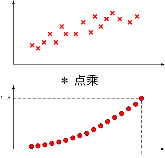
其中,\(\theta_t, \theta_{t-1}, \cdots , \theta_1\)表示原始数据集,即下图中的第一张图;
\((1-\beta), (1-\beta)\cdot \beta, \cdots, (1-\beta)\cdot \beta^{t-1}\)类似指数曲线,如下图中第二张图;从右向左,呈指数下降;
\(V_t\)表示两者点乘,将原始数据值与衰减指数点乘,相当于做了指数衰减,离的越近,影响就越大;离的越远,影响就越小,衰减就越严重;
2.2.2 实际计算指数加权平均
实际应用中,为了减少内存的使用,可以使用如下语句实现指数加权平均:
\(V_0=0\)
Repeat{
}
2.3 偏差修正(bias correction)
因为初始假设\(V_0=0\),可以想到,在使用\(V_t = \beta V_{t-1} + (1-\beta)\theta_t\)计算的时候,前面的一些值将会受到很大的影响,会比正常值小一些,直到计算后面数据的时候,影响才会渐渐变小,趋于正常。
因此,修正这种问题的方式是偏移修正(bias correction),即对\(V_t\)作如下处理:
在机器学习中,偏移修正不是必须的;
3. Gradient descent with momentum(Momentum梯度下降法)
动量梯度下降算法(Gradient descent with momentum)的速度要快于标准的梯度下降算法;
具体做法是:在每次训练时,对梯度计算指数加权平均,然后使用得到的梯度值更新权重和偏置;
3.1 梯度下降
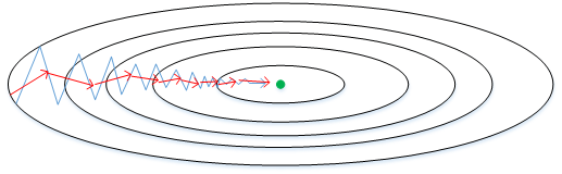
如上图蓝色折线所示,表示标准梯度下降算法;在梯度下降的过程中,会出现震荡的情况,这是因为每一点的梯度只与当前梯度方向有关,因此会出现折线的效果;
如上图红色折线所示,表示使用momentum梯度下降算法;可以看到,在梯度下降的过程中,不会出现剧烈的震荡,这是因为,每一个点的梯度不仅与当前梯度方向有关,还与之前的梯度方向有关;能够做到纵轴摆动变小,横轴方向运动更快;
3.2 伪代码表示
On iteration t{
Compute dW, db on the current mini-batch
\(V_{dW} = \beta V_{dW} + (1-\beta)dW\)
\(V_{db} = \beta V_{db} + (1-\beta)db\)
更新权重和偏置
\(W := W - \alpha V_{dW}, b := b - \alpha V_{db}\)
}
其中,初始化时,\(V_{dW}=0, V_{db}=0, \beta=0.9\);
3.3 TensorFlow中的Gradient descent with momentum
3.3.1 构建optimizer
# optimizer
optimizer = tf.train.MomentumOptimizer(0.01, momentum) # \beta
train = optimizer.minimize(loss)
3.3.2 tf.train.MomentumOptimizer()
tf.train.MomentumOptimizer.__init__(self, learning_rate, momentum,
               use_locking=False, name="Momentum", use_nesterov=False):

Args:
	learning_rat: A `Tensor` or a floating point value.  The learning rate. # 学习率
	momentum: A `Tensor` or a floating point value.  The momentum. # 就是指数加权平均中的超参数\alpha=0.9
	use_locking: If `True` use locks for update operations.
	name: Optional name prefix for the operations created when applying gradients.  Defaults to "Momentum".
	use_nesterov: If `True` use Nesterov Momentum. # 另一种优化算法,由momentum改进而来,效果更好;来源于:http://jmlr.org/proceedings/papers/v28/sutskever13.pdf

Return:
    optimizer
4. RMSprop
RMSprop(Root mean squared prop)是另外一种优化梯度下降的算法,类似于Momentum Gradient descent,同样可以在纵轴上减小摆动,在横轴方向上运动更快;
4.1 伪代码表示
On iteration t{
Compute dW, db on the current mini-batch
\(S_{dW} = \beta S_{dW} + (1-\beta)(dW)^2\)
\(S_{db} = \beta S_{db} + (1-\beta)(db)^2\)
更新权重和偏置
\(W := W - \alpha \dfrac{dW}{\sqrt{S_W}+\epsilon}, b := b - \alpha \dfrac{db}{\sqrt{S_W}+\epsilon}\)
}
其中,一般取\(\epsilon=10^{-8}\),防止分母趋近于0;
4.2 TensorFlow中的RMSprop
4.2.1 构建optimizer
# optimizer
optimizer = tf.train.RMSPropOptimizer(0.01, decay, momentum) # decay不清楚具体什么作用??求解:
train = optimizer.minimize(loss)
4.2.2 tf.train.RMSPropOptimizer()
tf.train.RMSPropOptimizer.__init__(self,
                                  learning_rate,
                                  decay=0.9,
                                  momentum=0.0,
                                  epsilon=1e-10,
                                  use_locking=False,
                                  centered=False,
                                  name="RMSProp")
Args:
	learning_rate: A Tensor or a floating point value.  The learning rate.  # 学习率
	decay: Discounting factor for the history/coming gradient  # ??
	momentum: A scalar tensor. # \alpha
	epsilon: Small value to avoid zero denominator.  # \epsilon 防止分母趋近于0
	use_locking: If True use locks for update operation.
	centered: If True, gradients are normalized by the estimated variance of the gradient; if False, by the uncentered second moment. Setting this to True may help with training, but is slightly more expensive in terms of computation and memory. Defaults to False.
	name: Optional name prefix for the operations created when applying gradients. Defaults to "RMSProp".
5. Adam optimization algorithm
Adam优化算法是结合了Gradient descent with momentum与RMSprop两种算法;被证明能够适用于不同的神经网络;
5.1 Adam算法流程-伪代码
初始化:\(V_{dW}=0, S_{dW}=0, V_{db}=0, S_{db}=0\);
On iteration t {
Compute \(dW, db\) on each mini-batch
\(V_{dW} = \beta_1 V_{dW} + (1-\beta_1)dW\)
\(V_{db} = \beta_1 V_{db} + (1-\beta_1)db\)
\(S_{dW} = \beta_2 S_{dW} + (1-\beta_2)(dW)^2\)
\(S_{db} = \beta_2 S_{db} + (1-\beta_2)(db)^2\)
\(V_{dW}^{corrected}= \dfrac{V_{dW}}{1-\beta_1^t}, V_{db}^{corrected}= \dfrac{V_{db}}{1-\beta_1^t}\)
\(S_{dW}^{corrected}= \dfrac{S_{dW}}{1-\beta_2^t}, S_{db}^{corrected}= \dfrac{S_{db}}{1-\beta_2^t}\)
\(W := W - \alpha \dfrac{V_{dW}^{corrected}}{\sqrt{S_{dW}^{corrected}}+\epsilon} b := b - \alpha \dfrac{V_{db}^{corrected}}{\sqrt{S_{db}^{corrected}}+\epsilon}\)
}
Adam算法中需要做偏差修正;
超参数设置:\(\beta_1 = 0.9, \beta_2=0.999, \epsilon = 10^{-8}\);一般只需要对学习率\(\alpha\)进行调试;
5.2 TensorFlow中Adam optimization algorithm
5.2.1 构建optimizer
optimizer = tf.train.AdamOptimizer(learning_rate, beta1, beta2, epsilon)
train = optimizer.minimize(loss)
5.2.2 tf.train.AdamOptimizer
tf.train.AdamOptimizer._init__(self,
                               learning_rate=0.001,
                               beta1=0.9,
                               beta2=0.999,
                               epsilon=1e-8,
                               use_locking=False,
                               name="Adam"):
Args:
	learning_rate: A Tensor or a floating point value.  The learning rate. # 学习率
	beta1: A float value or a constant float tensor. The exponential decay rate for the 1st moment estimates. # \beta_1
	beta2: A float value or a constant float tensor. The exponential decay rate for the 2nd moment estimates. # \beta_2
	epsilon: A small constant for numerical stability. This epsilon is "epsilon hat" in the Kingma and Ba paper (in the formula just before Section 2.1), not the epsilon in Algorithm 1 of the paper.
	use_locking: If True use locks for update operations.
	name: Optional name for the operations created when applying gradients. Defaults to "Adam".
6. 不同优化算法的优缺点总结
6.1 Batch Gradient Descent
思想:基于整个训练集进行梯度下降,更新权重;
优点:
- 考虑的是全局损失,不会陷入局部最优;
缺点:
- 每次迭代计算量较大,占用内存较高;
6.2 Stochastic Gradient Descent
思想:从训练集中随机选取一个样本计算梯度更新参数;
优点:
- 由于是对当个样本的损失计算梯度,因此计算量较小;
缺点:
- 仅考虑单个样本,容易陷入局部最优;
- 训练集较大时,训练时间较长;
- 选择合适的学习率比较困难;
- 对参数初始化比较敏感;
- 由于引入了噪声,因此具有正则化的效果;
6.3 Mini Batch Gradient Descent
思想:从整个样本集中选择batch_size个样本计算损失的梯度,更新权重;
优点:
- 对于很大的训练集,能够较快的收敛;
缺点:
- 梯度更新的方向依赖于当前batch内的样本,所以梯度的方向不稳定;
- 可能会出现不会收敛的最小值的情况,需要逐渐减小学习率;
6.4 Gradient Descent with Momentum
思想:基于之前梯度的方向以及当前batch的梯度方向进行更新;
优点:
- 减弱纵向方向的摆动,对震荡的情况能够有一定的抑制作用;
- 加速横向的运动,快速接近于最优值,加速收敛;
6.5 RMSprop
思想:类似于动量梯度下降,引入了指数权重加权平均值;
6.6 AdaGrad
思想:综合了Gradient Descent with Momentum与RMSprop两种优化算法;
优点:
- 训练前期,更新幅度大;
- 训练后期,更新幅度小;
- 适合处理稀疏梯度;
缺点:
- 训练后期,会导致学习率很小,梯度更新的很慢;
- 自定义全局学习率;
7. Learning rate decay
在神经网络训练的过程中,适当减小学习率有利于提高训练速度,该类方法称为learning rate decay,即随着迭代次数的增加,学习率\(\alpha\)逐渐减小;
7.1 学习率减小的几种方式
(1)第一种:
其中,\(decay\_rate\)衰减参数;\(epoch\_num\)表示迭代次数;
(2)第二种:
(3)第三种:
(4)第四种:
将\(\alpha\)设置为关于\(t\)的离散值,随着\(t\)的增加,\(\alpha\)呈阶梯式减少;
(5)第五种:
通过查看训练日志,手动调整学习率;
7.2 TensorFlow中的学习率设置
由于TensorFlow中提供的学习率设置方式有不少种,而本文主要是叙述梯度下降的优化算法,在此处介绍将会占用不小的篇幅,显得有些臃肿,因此,另总结一篇博文供自己学习;
8. The problem of local optima
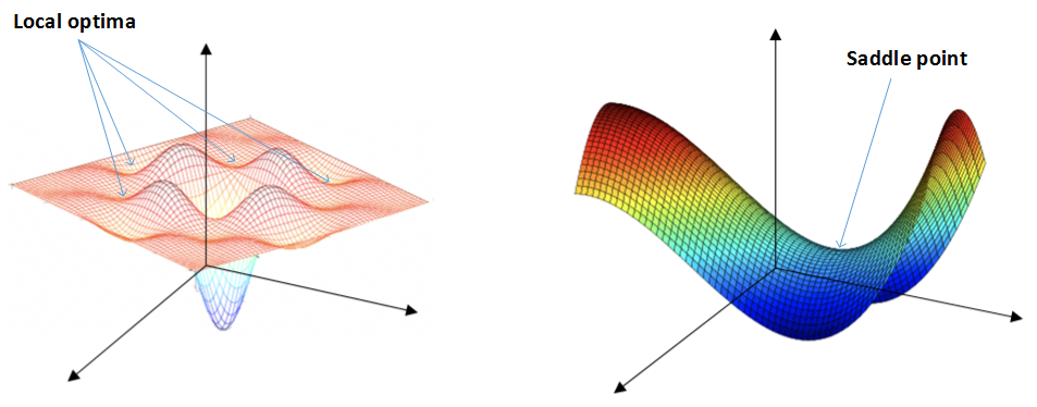
在使用梯度下降算法减少cost function的时候,可能会得到局部最优解,而不是全局最优解;
我们认为的局部最优可能如下图左边所示;但在神经网络中,局部最优的概念发生了变化;大部分梯度为零的“最优点“不是这些凹槽处,而是如下图右边的马鞍处,称为saddle point。
类似马鞍状的plateaus会降低神经网络的学习速度。plateaus是梯度接近于零的平缓区域,如下图所示,在plateaus上梯度很小,前进缓慢,达到saddle point需要很长时间;到达saddle point后,由于随机扰动,梯度能够进去下降;但是会在plateaus上花费很多时间;
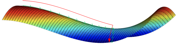
动量梯度下降、RMSprop、Adam算法能够解决plateaus下降过慢的问题,提高训练速度;
结束!!!
博主个人网站:https://chenzhen.online