kaggle 欺诈信用卡预测——不平衡训练样本的处理方法 综合结论就是:随机森林+过采样(直接复制或者smote后,黑白比例1:3 or 1:1)效果比较好!记得在smote前一定要先做标准化!!!其实随机森林对特征是否标准化无感,但是svm和LR就非常非常关键了

先看数据:

特征如下:
Time

Number of seconds elapsed between each transaction (over two days)

numeric
V1
No description provided
numeric
V2
No description provided
numeric
V3
No description provided
numeric
V4
No description provided
numeric
V5
No description provided
numeric
V6
No description provided
numeric
V7
No description provided
numeric
V8
No description provided
numeric
V9
No description provided
numeric
V10
No description provided
numeric
V11
No description provided
numeric
V12
No description provided
numeric
V13
No description provided
numeric
V14
No description provided
numeric
V15
No description provided
numeric
V16
No description provided
numeric
V17
No description provided
numeric
V18
No description provided
numeric
V19
No description provided
numeric
V20
No description provided
numeric
V21
No description provided
numeric
V22
No description provided
numeric
V23
No description provided
numeric
V24
No description provided
numeric
V25
No description provided
numeric
V26
No description provided
numeric
V27
No description provided
numeric
V28

abc

numeric
Amount

Amount of money for this transaction

numeric
Class

Fraud or Not-Fraud

boolean
只有Amount没有做标准化处理(mean不为0!!!):见:https://www.kaggle.com/mlg-ulb/creditcardfraud/data

Introduction

from:https://www.kaggle.com/nikitaivanov/getting-high-sensitivity-for-imbalanced-data 主要使用了smote和聚类两种思路!

In this notebook we will try to predict fraud transactions from a given data set. Given that the data is imbalanced, standard metrics for evaluating classification algorithm (such as accuracy) are invalid. We will focus on the following metrics: Sensitivity (true positive rate) and Specificity (true negative rate). Of course, they are dependent on each other, so we want to find optimal trade-off between them. Such trade-off usually depends on the application of the algorithm, and in case of fraud detection I would prefer to see high sensitivity (e.g. given that a transaction is fraud, I want to be able to detect it with high probability).

For dealing with skewed data I am going to use SMOTE algorithm. In two words, the idea is to create synthetic samples (in opposite to oversampling with replacement) through finding nearest examples (KNN), calculating difference between them, multiplying this difference by a random number between 0 and 1 and adding the result to the initial sample. For this purpose we are going to use SMOTE function from DMwR package.

Algorithms I am going to implement are Support Vector Machine (SVM), Logistic regression and Random Forest. Models will be trained on the original and SMOTEd data and their performance will be measured on the entire data set.

As a bonus, we are going to have some fun and use K-means centroids of the negative examples together with the original positive examples as a new dataset and train our algorithm on it. We then compare results.

 
##Loading required packeges 
library(ggplot2) #visualization  
library(caret) #train model
library(dplyr) #data manipulation
library(kernlab) #svm
library(nnet) #models (logit, neural nets)
library(DMwR) #SMOTE data

##Load data
d = read.csv("../input/creditcard.csv")
n = ncol(d)
str(d)
d$Class = ifelse(d$Class == 0, 'No', 'Yes') %>% as.factor()
 
Loading required package: lattice

Attaching package: ‘dplyr’

The following objects are masked from ‘package:stats’:

    filter, lag

The following objects are masked from ‘package:base’:

    intersect, setdiff, setequal, union


Attaching package: ‘kernlab’

The following object is masked from ‘package:ggplot2’:

    alpha

Loading required package: grid
'data.frame':	284807 obs. of  31 variables:
 $ Time  : num  0 0 1 1 2 2 4 7 7 9 ...
 $ V1    : num  -1.36 1.192 -1.358 -0.966 -1.158 ...
 $ V2    : num  -0.0728 0.2662 -1.3402 -0.1852 0.8777 ...
 $ V3    : num  2.536 0.166 1.773 1.793 1.549 ...
 $ V4    : num  1.378 0.448 0.38 -0.863 0.403 ...
 $ V5    : num  -0.3383 0.06 -0.5032 -0.0103 -0.4072 ...
 $ V6    : num  0.4624 -0.0824 1.8005 1.2472 0.0959 ...
 $ V7    : num  0.2396 -0.0788 0.7915 0.2376 0.5929 ...
 $ V8    : num  0.0987 0.0851 0.2477 0.3774 -0.2705 ...
 $ V9    : num  0.364 -0.255 -1.515 -1.387 0.818 ...
 $ V10   : num  0.0908 -0.167 0.2076 -0.055 0.7531 ...
 $ V11   : num  -0.552 1.613 0.625 -0.226 -0.823 ...
 $ V12   : num  -0.6178 1.0652 0.0661 0.1782 0.5382 ...
 $ V13   : num  -0.991 0.489 0.717 0.508 1.346 ...
 $ V14   : num  -0.311 -0.144 -0.166 -0.288 -1.12 ...
 $ V15   : num  1.468 0.636 2.346 -0.631 0.175 ...
 $ V16   : num  -0.47 0.464 -2.89 -1.06 -0.451 ...
 $ V17   : num  0.208 -0.115 1.11 -0.684 -0.237 ...
 $ V18   : num  0.0258 -0.1834 -0.1214 1.9658 -0.0382 ...
 $ V19   : num  0.404 -0.146 -2.262 -1.233 0.803 ...
 $ V20   : num  0.2514 -0.0691 0.525 -0.208 0.4085 ...
 $ V21   : num  -0.01831 -0.22578 0.248 -0.1083 -0.00943 ...
 $ V22   : num  0.27784 -0.63867 0.77168 0.00527 0.79828 ...
 $ V23   : num  -0.11 0.101 0.909 -0.19 -0.137 ...
 $ V24   : num  0.0669 -0.3398 -0.6893 -1.1756 0.1413 ...
 $ V25   : num  0.129 0.167 -0.328 0.647 -0.206 ...
 $ V26   : num  -0.189 0.126 -0.139 -0.222 0.502 ...
 $ V27   : num  0.13356 -0.00898 -0.05535 0.06272 0.21942 ...
 $ V28   : num  -0.0211 0.0147 -0.0598 0.0615 0.2152 ...
 $ Amount: num  149.62 2.69 378.66 123.5 69.99 ...
 $ Class : int  0 0 0 0 0 0 0 0 0 0 ...
 

It is always a good idea first to plot a response variable to check for skewness in data:

 
qplot(x = d$Class, geom = 'bar') + xlab('Fraud (Yes/No)') + ylab('Number of transactions')


Classification on the original data

Keeping in mind that the data is highly skewed we proceed. First split the data into training and test sets.

 
idx = createDataPartition(d$Class, p = 0.7, list = F)
d[, -n] = scale(d[, -n]) #perform scaling
train = d[idx, ]
test = d[-idx, ]
 

Calculate baseline accuracy for future reference

 
blacc = nrow(d[d$Class == 'No', ])/nrow(d)*100
cat('Baseline accuracy:', blacc)
 
Baseline accuracy: 99.82725
 

To begin with, let's train our models on the original dataset to see what we get if use unbalanced data. Due to computational limitations of my laptop, I will only run logistic regression for this purpose.

 
m1 = multinom(data = train, Class ~ .)
p1 = predict(m1, test[, -n], type = 'class')
cat(' Accuracy of the model', mean(p1 == test[, n])*100, '
', 'Baseline accuracy', blacc)
 
# weights:  32 (31 variable)
initial  value 138189.980799 
final  value 31315.159746 
converged
 Accuracy of the model 99.92744 
 Baseline accuracy 99.82725
 

Though accuracy (99.92%) of the model might look impressive at a first glance, in fact it isn't. Simply predicting 'not a fraud' for all transactions will give 99.83% accuracy. To really evaluate model's perfomance we need to check confusion matrix.

 
confusionMatrix(p1, test[, n], positive = 'Yes')
 
Confusion Matrix and Statistics

          Reference
Prediction    No   Yes
       No  85287    55
       Yes     7    92
                                          
               Accuracy : 0.9993          
                 95% CI : (0.9991, 0.9994)
    No Information Rate : 0.9983          
    P-Value [Acc > NIR] : 1.779e-15       
                                          
                  Kappa : 0.7476          
 Mcnemar's Test P-Value : 2.387e-09       
                                          
            Sensitivity : 0.625850        
            Specificity : 0.999918        
         Pos Pred Value : 0.929293        
         Neg Pred Value : 0.999356        
             Prevalence : 0.001720        
         Detection Rate : 0.001077        
   Detection Prevalence : 0.001159        
      Balanced Accuracy : 0.812884        
                                          
       'Positive' Class : Yes             


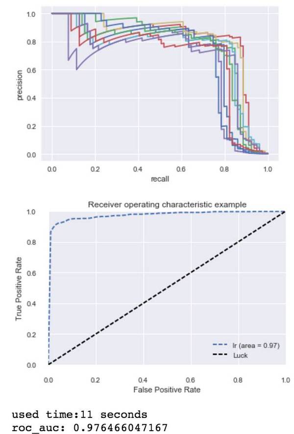
From the confusion matrix we see that while model has high accuracy (99.92%) and high specificity (99.98%), it has low sensitivity of 64%. In other words, only 64% of all fraudulent transactions were detected.


Classification on the SMOTEd data

Now let's preprocess our data using SMOTE algorithm:

 
table(d$Class) #check initial distribution
newData <- SMOTE(Class ~ ., d, perc.over = 500,perc.under=100)
table(newData$Class) #check SMOTed distribution
 
    No    Yes 
284315    492 
  No  Yes 
2460 2952 
 

To train SVM (with RBF kernel) we are going to use train function from caret package. It allows to choose optimal parameters of the model (cost and sigma in this case). Cost refers to penalty for misclassifying examples and sigma is a parameter of RBF which measures similarity between examples. To choose best model we use 5-fold cross-validation. We then evaluate our model on the entire data set.

 
gr = expand.grid(C = c(1, 50, 150), sigma = c(0.01, 0.05, 1))
tr = trainControl(method = 'cv', number = 5)
m2 = train(data = newData, Class ~ ., method = 'svmRadial', trControl = tr, tuneGrid = gr)
m2
 
Support Vector Machines with Radial Basis Function Kernel 

5412 samples
  30 predictor
   2 classes: 'No', 'Yes' 

No pre-processing
Resampling: Cross-Validated (5 fold) 
Summary of sample sizes: 4330, 4329, 4329, 4330, 4330 
Resampling results across tuning parameters:

  C    sigma  Accuracy   Kappa    
    1  0.01   0.9445668  0.8891865
    1  0.05   0.9626774  0.9250408
    1  1.00   0.9672934  0.9344234
   50  0.01   0.9717300  0.9430408
   50  0.05   0.9863262  0.9723782
   50  1.00   0.9695108  0.9388440
  150  0.01   0.9789351  0.9574955
  150  0.05   0.9850335  0.9697552
  150  1.00   0.9695108  0.9388440

Accuracy was used to select the optimal model using  the largest value.
The final values used for the model were sigma = 0.05 and C = 50. 
 

As wee see, best tuning parameters are C = 50 and sigma = 0.05

Let's look at a confusion matrix

 
p2 = predict(m2, d[, -n])
confusionMatrix(p2, d[, n], positive = 'Yes')
 
Confusion Matrix and Statistics

          Reference
Prediction     No    Yes
       No  278470      2
       Yes   5845    490
                                        
               Accuracy : 0.9795        
                 95% CI : (0.9789, 0.98)
    No Information Rate : 0.9983        
    P-Value [Acc > NIR] : 1             
                                        
                  Kappa : 0.1408        
 Mcnemar's Test P-Value : <2e-16        
                                        
            Sensitivity : 0.995935      
            Specificity : 0.979442      
         Pos Pred Value : 0.077348      
         Neg Pred Value : 0.999993      
             Prevalence : 0.001727      
         Detection Rate : 0.001720      
   Detection Prevalence : 0.022243      
      Balanced Accuracy : 0.987688      
                                        
       'Positive' Class : Yes           


(Numbers may differ due to randomness of k-fold cv)

As expected we were able to achieve sensitivity of 99.59%. In other words, out of all fraudulent transactions we correctly detected 99.59% of them. This came in price of slightly lower accuracy (in comparison to the first model) - 97.95% vs. 99.92% and lower specificity 97.94% vs. 99.98%. The main disadvantage is low level of positive predicted value (i.e. given that prediction is positive, what is probability that the true state is positive) which this case is 7.74% vs. 85% for initial (unbalanced dataset) model. As was mentioned in the beginning, one should choose a model that matches certain goals. If the goal is to correctly identify fraudulent transactions even in price of low positive predicted value (which I believe the case), then the latter model (based on SMOTed data) should be used. Looking at confusion matrix we see that almost all fraudulent transactions were correctly identified and only 2.5% were mislabeled as fraudulent.

I'm planning to try couple more models and also use more sophisticated algorithm that uses K-means centroids of the majority class as samples for non fraudulent transactions.

 
m3 = randomForest(data = newData, Class ~ .)
p3 = predict(m3, d[, -n])
confusionMatrix(p3, d[, n], positive = 'Yes')
 
Error in eval(expr, envir, enclos): could not find function "randomForest"
Traceback:
 
library(randomForest)
m3 = randomForest(data = newData, Class ~ .)
p3 = predict(m3, d[, -n])
confusionMatrix(p3, d[, n], positive = 'Yes')
 
randomForest 4.6-12
Type rfNews() to see new features/changes/bug fixes.

Attaching package: ‘randomForest’

The following object is masked from ‘package:dplyr’:

    combine

The following object is masked from ‘package:ggplot2’:

    margin

Confusion Matrix and Statistics

          Reference
Prediction     No    Yes
       No  282105      0
       Yes   2210    492
                                          
               Accuracy : 0.9922          
                 95% CI : (0.9919, 0.9926)
    No Information Rate : 0.9983          
    P-Value [Acc > NIR] : 1               
                                          
                  Kappa : 0.306           
 Mcnemar's Test P-Value : <2e-16          
                                          
            Sensitivity : 1.000000        
            Specificity : 0.992227        
         Pos Pred Value : 0.182087        
         Neg Pred Value : 1.000000        
             Prevalence : 0.001727        
         Detection Rate : 0.001727        
   Detection Prevalence : 0.009487        
      Balanced Accuracy : 0.996113        
                                          
       'Positive' Class : Yes             


Random forest performs really well. Sensitivity 100% and high specificity (more than 99%). All fraudulent transactions were detected and less than 1% of all transactions were falsely classified as fraud. Hence, Random Forest + SMOTE algorithm shloud be considered as final model.


K-means centroids as a new sample

For curiosity, let's take another approach in dealing with imbalanced data. We are going to separate the examples for positive and negative and from the latter one extract centroids (generated using K-means clustering). Number of clusters will be equal to the number of positive examples. We then use these centroids together with positive examples as a new sample.(思路就是聚类,将major class聚类为k个点,其中k为欺诈信用卡的样本数!)

 
neg = d[d$Class == 'No', ] #negative examples
pos = d[d$Class == 'Yes', ] #positive examples
n_pos = sum(d$Class == 'Yes') #calculate number of positive examples
clus = kmeans(neg[, -n], centers = n_pos, iter.max = 100) #perform K-means
neg = as.data.frame(clus$centers) #extract centroids as new sample
neg$Class = 'No'
newData = rbind(neg, pos) #merge positive and negative examples
newData$Class = factor(newData$Class)
 

We run random forest on the new dataset, newData, and check confusion matrix.

 
m4 = randomForest(data = newData, Class ~ .)
p4 = predict(m4, d[, -n])
confusionMatrix(p4, d[, n], positive = 'Yes')
 
Confusion Matrix and Statistics

          Reference
Prediction     No    Yes
       No  210086      0
       Yes  74229    492
                                         
               Accuracy : 0.7394         
                 95% CI : (0.7378, 0.741)
    No Information Rate : 0.9983         
    P-Value [Acc > NIR] : 1              
                                         
                  Kappa : 0.0097         
 Mcnemar's Test P-Value : <2e-16         
                                         
            Sensitivity : 1.000000       
            Specificity : 0.738920       
         Pos Pred Value : 0.006584       
         Neg Pred Value : 1.000000       
             Prevalence : 0.001727       
         Detection Rate : 0.001727       
   Detection Prevalence : 0.262357       
      Balanced Accuracy : 0.869460       
                                         
       'Positive' Class : Yes            


Well, while sensitivity is still 100%, specificity dropped to 72% leading to a big fraction of false positive predictions. Learning on the data that was transformed using SMOTE algorithm gave much better results.

from:https://www.kaggle.com/themlguy/undersample-and-oversample-approach-explored

 
# This Python 3 environment comes with many helpful analytics libraries installed
# It is defined by the kaggle/python docker image: https://github.com/kaggle/docker-python
# For example, here's several helpful packages to load in 

import numpy as np # linear algebra
import pandas as pd # data processing, CSV file I/O (e.g. pd.read_csv)

# Input data files are available in the "../input/" directory.
# For example, running this (by clicking run or pressing Shift+Enter) will list the files in the input directory

import os
print(os.listdir("../input"))

# Any results you write to the current directory are saved as output.
 
['creditcard.csv']
 
import matplotlib.pyplot as plt
from sklearn.cross_validation import train_test_split
from sklearn.linear_model import LogisticRegression
from sklearn.model_selection import GridSearchCV
from sklearn.svm import SVC
from sklearn.ensemble import RandomForestClassifier
from sklearn.preprocessing import StandardScaler
import seaborn as sns
from sklearn.metrics import confusion_matrix,recall_score,precision_recall_curve,auc,roc_curve,roc_auc_score,classification_report
 
/opt/conda/lib/python3.6/site-packages/sklearn/cross_validation.py:41: DeprecationWarning: This module was deprecated in version 0.18 in favor of the model_selection module into which all the refactored classes and functions are moved. Also note that the interface of the new CV iterators are different from that of this module. This module will be removed in 0.20.
  "This module will be removed in 0.20.", DeprecationWarning)
 
creditcard_data=pd.read_csv("../input/creditcard.csv")
 
creditcard_data['Amount']=StandardScaler().fit_transform(creditcard_data['Amount'].values.reshape(-1, 1))
creditcard_data.drop(['Time'], axis=1, inplace=True)
 
def generatePerformanceReport(clf,X_train,y_train,X_test,y_test,bool_):
    if bool_==True:
        clf.fit(X_train,y_train.values.ravel())
    pred=clf.predict(X_test)
    cnf_matrix=confusion_matrix(y_test,pred)
    tn, fp, fn, tp=cnf_matrix.ravel()
    print('---------------------------------')
    print('Length of training data:',len(X_train))
    print('Length of test data:', len(X_test))
    print('---------------------------------')
    print('True positives:',tp)
    print('True negatives:',tn)
    print('False positives:',fp)
    print('False negatives:',fn)
    #sns.heatmap(cnf_matrix,cmap="coolwarm_r",annot=True,linewidths=0.5)
    print('----------------------Classification report--------------------------')
    print(classification_report(y_test,pred))
    
 
#generate 50%, 66%, 75% proportions of normal indices to be combined with fraud indices 也就是说采样后的黑白样本比例是:0.5,0.66,0.75
#undersampled data
normal_indices=creditcard_data[creditcard_data['Class']==0].index
fraud_indices=creditcard_data[creditcard_data['Class']==1].index
for i in range(1,4):
    normal_sampled_data=np.array(np.random.choice(normal_indices, i*len(fraud_indices),replace=False)) #a random sample is generated from normal_indices 主要是随机欠采样
    undersampled_data=np.concatenate([fraud_indices, normal_sampled_data])
    undersampled_data=creditcard_data.iloc[undersampled_data]
    print('length of undersampled data ', len(undersampled_data))
    print('% of fraud transactions in undersampled data ',len(undersampled_data.loc[undersampled_data['Class']==1])/len(undersampled_data))
    #get feature and label data
    feature_data=undersampled_data.loc[:,undersampled_data.columns!='Class']
    label_data=undersampled_data.loc[:,undersampled_data.columns=='Class']
    X_train, X_test, y_train, y_test=train_test_split(feature_data,label_data,test_size=0.30)
    for j in [LogisticRegression(),SVC(),RandomForestClassifier(n_estimators=100)]:
        clf=j
        print(j)
        generatePerformanceReport(clf,X_train,y_train,X_test,y_test,True)
        #the above code classifies X_test which is part of undersampled data
        #now, let us consider the remaining rows of dataset and use that as test set
        remaining_indices=[i for i in creditcard_data.index  if i not in undersampled_data.index]
        testdf=creditcard_data.iloc[remaining_indices]
        testdf_label=creditcard_data.loc[:,testdf.columns=='Class']
        testdf_feature=creditcard_data.loc[:,testdf.columns!='Class']
        generatePerformanceReport(clf,X_train,y_train,testdf_feature,testdf_label,False)
 
length of undersampled data  984
% of fraud transactions in undersampled data  0.5
LogisticRegression(C=1.0, class_weight=None, dual=False, fit_intercept=True,
          intercept_scaling=1, max_iter=100, multi_class='ovr', n_jobs=1,
          penalty='l2', random_state=None, solver='liblinear', tol=0.0001,
          verbose=0, warm_start=False)
---------------------------------
Length of training data: 688
Length of test data: 296
---------------------------------
True positives: 144
True negatives: 134
False positives: 11
False negatives: 7
----------------------Classification report--------------------------
             precision    recall  f1-score   support

          0       0.95      0.92      0.94       145
          1       0.93      0.95      0.94       151

avg / total       0.94      0.94      0.94       296

---------------------------------
Length of training data: 688
Length of test data: 284807
---------------------------------
True positives: 461
True negatives: 270879
False positives: 13436
False negatives: 31
----------------------Classification report--------------------------
             precision    recall  f1-score   support

          0       1.00      0.95      0.98    284315
          1       0.03      0.94      0.06       492 #可以看到LR在测试数据集上表现并不好

avg / total       1.00      0.95      0.97    284807

SVC(C=1.0, cache_size=200, class_weight=None, coef0=0.0,
  decision_function_shape='ovr', degree=3, gamma='auto', kernel='rbf',
  max_iter=-1, probability=False, random_state=None, shrinking=True,
  tol=0.001, verbose=False)
---------------------------------
Length of training data: 688
Length of test data: 296
---------------------------------
True positives: 144
True negatives: 140
False positives: 5
False negatives: 7
----------------------Classification report--------------------------
             precision    recall  f1-score   support

          0       0.95      0.97      0.96       145
          1       0.97      0.95      0.96       151

avg / total       0.96      0.96      0.96       296

---------------------------------
Length of training data: 688
Length of test data: 284807
---------------------------------
True positives: 463
True negatives: 267084
False positives: 17231
False negatives: 29
----------------------Classification report--------------------------
             precision    recall  f1-score   support

          0       1.00      0.94      0.97    284315
          1       0.03      0.94      0.05       492 #看来svm在测试数据集上也不行啊

avg / total       1.00      0.94      0.97    284807

RandomForestClassifier(bootstrap=True, class_weight=None, criterion='gini',
            max_depth=None, max_features='auto', max_leaf_nodes=None,
            min_impurity_decrease=0.0, min_impurity_split=None,
            min_samples_leaf=1, min_samples_split=2,
            min_weight_fraction_leaf=0.0, n_estimators=100, n_jobs=1,
            oob_score=False, random_state=None, verbose=0,
            warm_start=False)
---------------------------------
Length of training data: 688
Length of test data: 296
---------------------------------
True positives: 144
True negatives: 142
False positives: 3
False negatives: 7
----------------------Classification report--------------------------
             precision    recall  f1-score   support

          0       0.95      0.98      0.97       145
          1       0.98      0.95      0.97       151

avg / total       0.97      0.97      0.97       296

---------------------------------
Length of training data: 688
Length of test data: 284807
---------------------------------
True positives: 485
True negatives: 275060
False positives: 9255
False negatives: 7
----------------------Classification report--------------------------
             precision    recall  f1-score   support

          0       1.00      0.97      0.98    284315
          1       0.05      0.99      0.09       492 #Rf也不行????

avg / total       1.00      0.97      0.98    284807

length of undersampled data  1476
% of fraud transactions in undersampled data  0.3333333333333333
LogisticRegression(C=1.0, class_weight=None, dual=False, fit_intercept=True,
          intercept_scaling=1, max_iter=100, multi_class='ovr', n_jobs=1,
          penalty='l2', random_state=None, solver='liblinear', tol=0.0001,
          verbose=0, warm_start=False)
---------------------------------
Length of training data: 1033
Length of test data: 443
---------------------------------
True positives: 130
True negatives: 291
False positives: 5
False negatives: 17
----------------------Classification report--------------------------
             precision    recall  f1-score   support

          0       0.94      0.98      0.96       296
          1       0.96      0.88      0.92       147

avg / total       0.95      0.95      0.95       443

---------------------------------
Length of training data: 1033
Length of test data: 284807
---------------------------------
True positives: 442
True negatives: 278887
False positives: 5428
False negatives: 50
----------------------Classification report--------------------------
             precision    recall  f1-score   support

          0       1.00      0.98      0.99    284315
          1       0.08      0.90      0.14       492

avg / total       1.00      0.98      0.99    284807

SVC(C=1.0, cache_size=200, class_weight=None, coef0=0.0,
  decision_function_shape='ovr', degree=3, gamma='auto', kernel='rbf',
  max_iter=-1, probability=False, random_state=None, shrinking=True,
  tol=0.001, verbose=False)
---------------------------------
Length of training data: 1033
Length of test data: 443
---------------------------------
True positives: 133
True negatives: 286
False positives: 10
False negatives: 14
----------------------Classification report--------------------------
             precision    recall  f1-score   support

          0       0.95      0.97      0.96       296
          1       0.93      0.90      0.92       147

avg / total       0.95      0.95      0.95       443

---------------------------------
Length of training data: 1033
Length of test data: 284807
---------------------------------
True positives: 453
True negatives: 274909
False positives: 9406
False negatives: 39
----------------------Classification report--------------------------
             precision    recall  f1-score   support

          0       1.00      0.97      0.98    284315
          1       0.05      0.92      0.09       492

avg / total       1.00      0.97      0.98    284807

RandomForestClassifier(bootstrap=True, class_weight=None, criterion='gini',
            max_depth=None, max_features='auto', max_leaf_nodes=None,
            min_impurity_decrease=0.0, min_impurity_split=None,
            min_samples_leaf=1, min_samples_split=2,
            min_weight_fraction_leaf=0.0, n_estimators=100, n_jobs=1,
            oob_score=False, random_state=None, verbose=0,
            warm_start=False)
---------------------------------
Length of training data: 1033
Length of test data: 443
---------------------------------
True positives: 128
True negatives: 293
False positives: 3
False negatives: 19
----------------------Classification report--------------------------
             precision    recall  f1-score   support

          0       0.94      0.99      0.96       296
          1       0.98      0.87      0.92       147

avg / total       0.95      0.95      0.95       443

---------------------------------
Length of training data: 1033
Length of test data: 284807
---------------------------------
True positives: 473
True negatives: 281560
False positives: 2755
False negatives: 19
----------------------Classification report--------------------------
             precision    recall  f1-score   support

          0       1.00      0.99      1.00    284315
          1       0.15      0.96      0.25       492

avg / total       1.00      0.99      0.99    284807

length of undersampled data  1968
% of fraud transactions in undersampled data  0.25
LogisticRegression(C=1.0, class_weight=None, dual=False, fit_intercept=True,
          intercept_scaling=1, max_iter=100, multi_class='ovr', n_jobs=1,
          penalty='l2', random_state=None, solver='liblinear', tol=0.0001,
          verbose=0, warm_start=False)
---------------------------------
Length of training data: 1377
Length of test data: 591
---------------------------------
True positives: 116
True negatives: 451
False positives: 5
False negatives: 19
----------------------Classification report--------------------------
             precision    recall  f1-score   support

          0       0.96      0.99      0.97       456
          1       0.96      0.86      0.91       135

avg / total       0.96      0.96      0.96       591

---------------------------------
Length of training data: 1377
Length of test data: 284807
---------------------------------
True positives: 433
True negatives: 282245
False positives: 2070
False negatives: 59
----------------------Classification report--------------------------
             precision    recall  f1-score   support

          0       1.00      0.99      1.00    284315
          1       0.17      0.88      0.29       492

avg / total       1.00      0.99      1.00    284807

SVC(C=1.0, cache_size=200, class_weight=None, coef0=0.0,
  decision_function_shape='ovr', degree=3, gamma='auto', kernel='rbf',
  max_iter=-1, probability=False, random_state=None, shrinking=True,
  tol=0.001, verbose=False)
---------------------------------
Length of training data: 1377
Length of test data: 591
---------------------------------
True positives: 118
True negatives: 447
False positives: 9
False negatives: 17
----------------------Classification report--------------------------
             precision    recall  f1-score   support

          0       0.96      0.98      0.97       456
          1       0.93      0.87      0.90       135

avg / total       0.96      0.96      0.96       591

---------------------------------
Length of training data: 1377
Length of test data: 284807
---------------------------------
True positives: 445
True negatives: 279369
False positives: 4946
False negatives: 47
----------------------Classification report--------------------------
             precision    recall  f1-score   support

          0       1.00      0.98      0.99    284315
          1       0.08      0.90      0.15       492

avg / total       1.00      0.98      0.99    284807

RandomForestClassifier(bootstrap=True, class_weight=None, criterion='gini',
            max_depth=None, max_features='auto', max_leaf_nodes=None,
            min_impurity_decrease=0.0, min_impurity_split=None,
            min_samples_leaf=1, min_samples_split=2,
            min_weight_fraction_leaf=0.0, n_estimators=100, n_jobs=1,
            oob_score=False, random_state=None, verbose=0,
            warm_start=False)
---------------------------------
Length of training data: 1377
Length of test data: 591
---------------------------------
True positives: 112
True negatives: 455
False positives: 1
False negatives: 23
----------------------Classification report--------------------------
             precision    recall  f1-score   support

          0       0.95      1.00      0.97       456
          1       0.99      0.83      0.90       135

avg / total       0.96      0.96      0.96       591

---------------------------------
Length of training data: 1377
Length of test data: 284807
---------------------------------
True positives: 469
True negatives: 283466
False positives: 849
False negatives: 23
----------------------Classification report--------------------------
             precision    recall  f1-score   support

          0       1.00      1.00      1.00    284315
          1       0.36      0.95      0.52       492

avg / total       1.00      1.00      1.00    284807

整体来看,因为欠采样只是用了一个模型,因此预测效果很差!!!因为没有用到全量数据特征,所以在全部数据集上表现并不好!
 
#oversampled_data data
normal_sampled_indices=creditcard_data.loc[creditcard_data['Class']==0].index
oversampled_data=creditcard_data.iloc[normal_sampled_indices]
fraud_data=creditcard_data.loc[creditcard_data['Class']==1]
oversampled_data=oversampled_data.append([fraud_data]*300, ignore_index=True) #此处过采样处理是直接将欺诈样本复制300份!!!
print('length of oversampled_data data ', len(oversampled_data))
print('% of fraud transactions in oversampled_data data ',len(oversampled_data.loc[oversampled_data['Class']==1])/len(oversampled_data))
#get feature and label data
feature_data=oversampled_data.loc[:,oversampled_data.columns!='Class']
label_data=oversampled_data.loc[:,oversampled_data.columns=='Class']
X_train, X_test, y_train, y_test=train_test_split(feature_data,label_data,test_size=0.30)
for j in [LogisticRegression(),RandomForestClassifier(n_estimators=100)]:
    clf=j
    print(j)
    generatePerformanceReport(clf,X_train,y_train,X_test,y_test,True)
    #the above code classifies X_test which is part of undersampled data
    #now, let us consider the remaining rows of dataset and use that as test set
    remaining_indices=[i for i in creditcard_data.index  if i not in oversampled_data.index]
    testdf=creditcard_data.iloc[remaining_indices]
    testdf_label=creditcard_data.loc[:,testdf.columns=='Class']
    testdf_feature=creditcard_data.loc[:,testdf.columns!='Class']
    generatePerformanceReport(clf,X_train,y_train,testdf_feature,testdf_label,False)
 
length of oversampled_data data  431915
% of fraud transactions in oversampled_data data  0.3417339059768704 最后复制后的欺诈样本比例为白样本的33%
LogisticRegression(C=1.0, class_weight=None, dual=False, fit_intercept=True,
          intercept_scaling=1, max_iter=100, multi_class='ovr', n_jobs=1,
          penalty='l2', random_state=None, solver='liblinear', tol=0.0001,
          verbose=0, warm_start=False)
---------------------------------
Length of training data: 302340
Length of test data: 129575
---------------------------------
True positives: 39803
True negatives: 84311
False positives: 1027
False negatives: 4434
----------------------Classification report--------------------------
             precision    recall  f1-score   support

          0       0.95      0.99      0.97     85338
          1       0.97      0.90      0.94     44237

avg / total       0.96      0.96      0.96    129575

---------------------------------
Length of training data: 302340
Length of test data: 284807
---------------------------------
True positives: 444
True negatives: 281055
False positives: 3260
False negatives: 48
----------------------Classification report--------------------------
             precision    recall  f1-score   support

          0       1.00      0.99      0.99    284315
          1       0.12      0.90      0.21       492 #效果也不咋的啊!

avg / total       1.00      0.99      0.99    284807

RandomForestClassifier(bootstrap=True, class_weight=None, criterion='gini',
            max_depth=None, max_features='auto', max_leaf_nodes=None,
            min_impurity_decrease=0.0, min_impurity_split=None,
            min_samples_leaf=1, min_samples_split=2,
            min_weight_fraction_leaf=0.0, n_estimators=100, n_jobs=1,
            oob_score=False, random_state=None, verbose=0,
            warm_start=False)
---------------------------------
Length of training data: 302340
Length of test data: 129575
---------------------------------
True positives: 44237
True negatives: 85327
False positives: 11
False negatives: 0
----------------------Classification report--------------------------
             precision    recall  f1-score   support

          0       1.00      1.00      1.00     85338
          1       1.00      1.00      1.00     44237

avg / total       1.00      1.00      1.00    129575

---------------------------------
Length of training data: 302340
Length of test data: 284807
---------------------------------
True positives: 492
True negatives: 284304
False positives: 11
False negatives: 0
----------------------Classification report--------------------------
             precision    recall  f1-score   support

          0       1.00      1.00      1.00    284315
          1       0.98      1.00      0.99       492 #随机森林还是不错的!!!

avg / total       1.00      1.00      1.00    284807


Random forest classifier with oversampled approach performs better compared to undersampled approach!!!

from:https://www.kaggle.com/gargmanish/how-to-handle-imbalance-data-study-in-detail

Hi all as we know credit card fraud detection will have a imbalanced data i.e having more number of normal class than the number of fraud class

In this I will use Basic method of handling imbalance data which are

This all I have done by using Analytics Vidya's blog please find the link Analytics Vidya

Undersampling:- it means taking the less number of majority class (In our case taking less number of Normal transactions so that our new data will be balanced

Oversampling: it means using replicating the data of minority class (fraud class) so that we can have a balanced data

SMOTE: it is also a type of oversampling but in this we will make the synthetic example of Minority data and will give as a balanced data

First I will start with the Undersampling and will try to classify using these Models

  1. Decision Tree Classifier/ Random Forest Classifier

  2. Logistic regression

  3. SVM

  4. XGboost

 
# This Python 3 environment comes with many helpful analytics libraries installed
# It is defined by the kaggle/python docker image: https://github.com/kaggle/docker-python
# For example, here's several helpful packages to load in 

import numpy as np # linear algebra
import pandas as pd # data processing, CSV file I/O (e.g. pd.read_csv)

# Input data files are available in the "../input/" directory.
# For example, running this (by clicking run or pressing Shift+Enter) will list the files in the input directory

from subprocess import check_output
print(check_output(["ls", "../input"]).decode("utf8"))

# Any results you write to the current directory are saved as output.
 
creditcard.csv


Lets start with Importing Libraries and data

 
import pandas as pd # to import csv and for data manipulation
import matplotlib.pyplot as plt # to plot graph
import seaborn as sns # for intractve graphs
import numpy as np # for linear algebra
import datetime # to dela with date and time
%matplotlib inline
from sklearn.preprocessing import StandardScaler # for preprocessing the data
from sklearn.ensemble import RandomForestClassifier # Random forest classifier
from sklearn.tree import DecisionTreeClassifier # for Decision Tree classifier
from sklearn.svm import SVC # for SVM classification
from sklearn.linear_model import LogisticRegression
from sklearn.cross_validation import train_test_split # to split the data
from sklearn.cross_validation import KFold # For cross vbalidation
from sklearn.model_selection import GridSearchCV # for tunnig hyper parameter it will use all combination of given parameters
from sklearn.model_selection import RandomizedSearchCV # same for tunning hyper parameter but will use random combinations of parameters
from sklearn.metrics import confusion_matrix,recall_score,precision_recall_curve,auc,roc_curve,roc_auc_score,classification_report
import warnings
warnings.filterwarnings('ignore')
 
/opt/conda/lib/python3.6/site-packages/sklearn/cross_validation.py:43: DeprecationWarning: This module was deprecated in version 0.18 in favor of the model_selection module into which all the refactored classes and functions are moved. Also note that the interface of the new CV iterators are different from that of this module. This module will be removed in 0.20.
  "This module will be removed in 0.20.", DeprecationWarning)
 
data = pd.read_csv("../input/creditcard.csv",header = 0)
 

Now explore the data to get insight in it

 
data.info()
 
<class 'pandas.core.frame.DataFrame'>
RangeIndex: 284807 entries, 0 to 284806
Data columns (total 31 columns):
Time      284807 non-null float64
V1        284807 non-null float64
V2        284807 non-null float64
V3        284807 non-null float64
V4        284807 non-null float64
V5        284807 non-null float64
V6        284807 non-null float64
V7        284807 non-null float64
V8        284807 non-null float64
V9        284807 non-null float64
V10       284807 non-null float64
V11       284807 non-null float64
V12       284807 non-null float64
V13       284807 non-null float64
V14       284807 non-null float64
V15       284807 non-null float64
V16       284807 non-null float64
V17       284807 non-null float64
V18       284807 non-null float64
V19       284807 non-null float64
V20       284807 non-null float64
V21       284807 non-null float64
V22       284807 non-null float64
V23       284807 non-null float64
V24       284807 non-null float64
V25       284807 non-null float64
V26       284807 non-null float64
V27       284807 non-null float64
V28       284807 non-null float64
Amount    284807 non-null float64
Class     284807 non-null int64
dtypes: float64(30), int64(1)
memory usage: 67.4 MB
 
  1. Hence we can see there are 284,807 rows and 31 columns which is a huge data
  2. Time is also in float here mean it can be only seconds starting from a particular time
 
# Now lets check the class distributions
sns.countplot("Class",data=data)
 
<matplotlib.axes._subplots.AxesSubplot at 0x7f6dabaaf128>
 
  1. As we know data is imbalanced and this graph also confirmed it
 
# now let us check in the number of Percentage
Count_Normal_transacation = len(data[data["Class"]==0]) # normal transaction are repersented by 0
Count_Fraud_transacation = len(data[data["Class"]==1]) # fraud by 1
Percentage_of_Normal_transacation = Count_Normal_transacation/(Count_Normal_transacation+Count_Fraud_transacation)
print("percentage of normal transacation is",Percentage_of_Normal_transacation*100)
Percentage_of_Fraud_transacation= Count_Fraud_transacation/(Count_Normal_transacation+Count_Fraud_transacation)
print("percentage of fraud transacation",Percentage_of_Fraud_transacation*100)
 
原始数据样本就是:500:1
percentage of normal transacation is 99.82725143693798
percentage of fraud transacation 0.1727485630620034
 
  1. Hence in data there is only 0.17 % are the fraud transcation while 99.83 are valid transcation
  2. So now we have to do resampling of this data
  3. before doing resampling lets have look at the amount related to valid transcation and fraud transcation
 
Fraud_transacation = data[data["Class"]==1]
Normal_transacation= data[data["Class"]==0]
plt.figure(figsize=(10,6))
plt.subplot(121)
Fraud_transacation.Amount.plot.hist(title="Fraud Transacation")
plt.subplot(122)
Normal_transacation.Amount.plot.hist(title="Normal Transaction")
 
<matplotlib.axes._subplots.AxesSubplot at 0x7f6da691cf60>
 
# the distribution for Normal transction is not clear and it seams that all transaction are less than 2.5 K
# So plot graph for same 
Fraud_transacation = data[data["Class"]==1]
Normal_transacation= data[data["Class"]==0]
plt.figure(figsize=(10,6))
plt.subplot(121)
Fraud_transacation[Fraud_transacation["Amount"]<= 2500].Amount.plot.hist(title="Fraud Tranascation")
plt.subplot(122)
Normal_transacation[Normal_transacation["Amount"]<=2500].Amount.plot.hist(title="Normal Transaction")
 
<matplotlib.axes._subplots.AxesSubplot at 0x7f6d98ecb0f0>
 
  1. Here now after exploring data we can say there is no pattern in data
  2. Now lets start with resmapling of data
 

ReSampling - Under Sampling


Before re sampling lets have look at the different accuracy matrices

Accuracy = TP+TN/Total

Precison = TP/(TP+FP)

Recall = TP/(TP+FN)

TP = True possitive means no of possitve cases which are predicted possitive

TN = True negative means no of negative cases which are predicted negative

FP = False possitve means no of negative cases which are predicted possitive

FN= False Negative means no of possitive cases which are predicted negative

Now for our case recall will be a better option because in these case no of normal transacations will be very high than the no of fraud cases and sometime a fraud case will be predicted as normal. So, recall will give us a sense of only fraud cases

Resampling

in this we will resample our data with different size

then we will try to use this resampled data to train our model

then we will use this model to predict for our original data

 
# for undersampling we need a portion of majority class and will take whole data of minority class
# count fraud transaction is the total number of fraud transaction
# now lets us see the index of fraud cases
fraud_indices= np.array(data[data.Class==1].index)
normal_indices = np.array(data[data.Class==0].index)
#now let us a define a function for make undersample data with different proportion
#different proportion means with different proportion of normal classes of data
def undersample(normal_indices,fraud_indices,times):#times denote the normal data = times*fraud data
    Normal_indices_undersample = np.array(np.random.choice(normal_indices,(times*Count_Fraud_transacation),replace=False)) #和上面例子是一样的!!!
    undersample_data= np.concatenate([fraud_indices,Normal_indices_undersample])
    undersample_data = data.iloc[undersample_data,:]
    
    print("the normal transacation proportion is :",len(undersample_data[undersample_data.Class==0])/len(undersample_data[undersample_data.Class]))
    print("the fraud transacation proportion is :",len(undersample_data[undersample_data.Class==1])/len(undersample_data[undersample_data.Class]))
    print("total number of record in resampled data is:",len(undersample_data[undersample_data.Class]))
    return(undersample_data)
 
## first make a model function for modeling with confusion matrix
def model(model,features_train,features_test,labels_train,labels_test):
    clf= model
    clf.fit(features_train,labels_train.values.ravel())
    pred=clf.predict(features_test)
    cnf_matrix=confusion_matrix(labels_test,pred)
    print("the recall for this model is :",cnf_matrix[1,1]/(cnf_matrix[1,1]+cnf_matrix[1,0]))
    fig= plt.figure(figsize=(6,3))# to plot the graph
    print("TP",cnf_matrix[1,1,]) # no of fraud transaction which are predicted fraud
    print("TN",cnf_matrix[0,0]) # no. of normal transaction which are predited normal
    print("FP",cnf_matrix[0,1]) # no of normal transaction which are predicted fraud
    print("FN",cnf_matrix[1,0]) # no of fraud Transaction which are predicted normal
    sns.heatmap(cnf_matrix,cmap="coolwarm_r",annot=True,linewidths=0.5)
    plt.title("Confusion_matrix")
    plt.xlabel("Predicted_class")
    plt.ylabel("Real class")
    plt.show()
    print("
----------Classification Report------------------------------------")
    print(classification_report(labels_test,pred))
    
 
def data_prepration(x): # preparing data for training and testing as we are going to use different data 
    #again and again so make a function
    x_features= x.ix[:,x.columns != "Class"]
    x_labels=x.ix[:,x.columns=="Class"]
    x_features_train,x_features_test,x_labels_train,x_labels_test = train_test_split(x_features,x_labels,test_size=0.3) #30%用于测试
    print("length of training data")
    print(len(x_features_train))
    print("length of test data")
    print(len(x_features_test))
    return(x_features_train,x_features_test,x_labels_train,x_labels_test)
 
# before starting we should standridze our ampount column
data["Normalized Amount"] = StandardScaler().fit_transform(data['Amount'].reshape(-1, 1))
data.drop(["Time","Amount"],axis=1,inplace=True)
data.head()
 
 V1V2V3V4V5V6V7V8V9V10...V21V22V23V24V25V26V27V28ClassNormalized Amount
0 -1.359807 -0.072781 2.536347 1.378155 -0.338321 0.462388 0.239599 0.098698 0.363787 0.090794 ... -0.018307 0.277838 -0.110474 0.066928 0.128539 -0.189115 0.133558 -0.021053 0 0.244964
1 1.191857 0.266151 0.166480 0.448154 0.060018 -0.082361 -0.078803 0.085102 -0.255425 -0.166974 ... -0.225775 -0.638672 0.101288 -0.339846 0.167170 0.125895 -0.008983 0.014724 0 -0.342475
2 -1.358354 -1.340163 1.773209 0.379780 -0.503198 1.800499 0.791461 0.247676 -1.514654 0.207643 ... 0.247998 0.771679 0.909412 -0.689281 -0.327642 -0.139097 -0.055353 -0.059752 0 1.160686
3 -0.966272 -0.185226 1.792993 -0.863291 -0.010309 1.247203 0.237609 0.377436 -1.387024 -0.054952 ... -0.108300 0.005274 -0.190321 -1.175575 0.647376 -0.221929 0.062723 0.061458 0 0.140534
4 -1.158233 0.877737 1.548718 0.403034 -0.407193 0.095921 0.592941 -0.270533 0.817739 0.753074 ... -0.009431 0.798278 -0.137458 0.141267 -0.206010 0.502292 0.219422 0.215153 0 -0.073403

5 rows × 30 columns


Logistic Regression with Undersample Data

 
# Now make undersample data with differnt portion
# here i will take normal trasaction in  0..5 %, 0.66% and 0.75 % proportion of total data now do this for 
for i in range(1,4):
    print("the undersample data for {} proportion".format(i))
    print()
    Undersample_data = undersample(normal_indices,fraud_indices,i)
    print("------------------------------------------------------------")
    print()
    print("the model classification for {} proportion".format(i))
    print()
    undersample_features_train,undersample_features_test,undersample_labels_train,undersample_labels_test=data_prepration(Undersample_data)
    print()
    clf=LogisticRegression()
    model(clf,undersample_features_train,undersample_features_test,undersample_labels_train,undersample_labels_test)
    print("________________________________________________________________________________________________________")
    
# here 1st proportion conatain 50% normal transaction
#Proportion 2nd contains 66% noraml transaction
#proportion 3rd contains 75 % normal transaction
 
the undersample data for 1 proportion

the normal transacation proportion is : 0.5
the fraud transacation proportion is : 0.5
total number of record in resampled data is: 984
------------------------------------------------------------

the model classification for 1 proportion

length of training data
688
length of test data
296

the recall for this model is : 0.897260273973
TP 131
TN 147
FP 3
FN 15
----------Classification Report------------------------------------
             precision    recall  f1-score   support

          0       0.91      0.98      0.94       150
          1       0.98      0.90      0.94       146 #测试集上???咋会这么高!!!

avg / total       0.94      0.94      0.94       296

________________________________________________________________________________________________________
the undersample data for 2 proportion

the normal transacation proportion is : 0.6666666666666666
the fraud transacation proportion is : 0.3333333333333333
total number of record in resampled data is: 1476
------------------------------------------------------------

the model classification for 2 proportion

length of training data
1033
length of test data
443

the recall for this model is : 0.929078014184
TP 131
TN 296
FP 6
FN 10
----------Classification Report------------------------------------
             precision    recall  f1-score   support

          0       0.97      0.98      0.97       302
          1       0.96      0.93      0.94       141

avg / total       0.96      0.96      0.96       443

________________________________________________________________________________________________________
the undersample data for 3 proportion

the normal transacation proportion is : 0.75
the fraud transacation proportion is : 0.25
total number of record in resampled data is: 1968
------------------------------------------------------------

the model classification for 3 proportion

length of training data
1377
length of test data
591

the recall for this model is : 0.892086330935
TP 124
TN 446
FP 6
FN 15
----------Classification Report------------------------------------
             precision    recall  f1-score   support

          0       0.97      0.99      0.98       452
          1       0.95      0.89      0.92       139

avg / total       0.96      0.96      0.96       591

________________________________________________________________________________________________________
 
  1. As the number of normal transaction is increasing the recall for fraud transcation is decreasing
  2. TP = no of fraud transaction which are predicted fraud
  3. TN = no. of normal transaction which are predicted normal
  4. FP = no of normal transaction which are predicted fraud
  5. FN =no of fraud Transaction which are predicted normal
 
#let us train this model using undersample data and test for the whole data test set #用欠采样训练的模型来预测全量数据集
for i in range(1,4):
    print("the undersample data for {} proportion".format(i))
    print()
    Undersample_data = undersample(normal_indices,fraud_indices,i)
    print("------------------------------------------------------------")
    print()
    print("the model classification for {} proportion".format(i))
    print()
    undersample_features_train,undersample_features_test,undersample_labels_train,undersample_labels_test=data_prepration(Undersample_data)
    data_features_train,data_features_test,data_labels_train,data_labels_test=data_prepration(data) 
    #the partion for whole data
    print()
    clf=LogisticRegression()
    model(clf,undersample_features_train,data_features_test,undersample_labels_train,data_labels_test)
    # here training for the undersample data but tatsing for whole data
    print("_________________________________________________________________________________________")
 
the undersample data for 1 proportion

the normal transacation proportion is : 0.5
the fraud transacation proportion is : 0.5
total number of record in resampled data is: 984
------------------------------------------------------------

the model classification for 1 proportion

length of training data
688
length of test data
296
length of training data
199364
length of test data
85443

the recall for this model is : 0.923076923077
TP 132
TN 81568
FP 3732
FN 11
----------Classification Report------------------------------------
             precision    recall  f1-score   support

          0       1.00      0.96      0.98     85300
          1       0.03      0.92      0.07       143 #果然是预测全量数据不好!!!

avg / total       1.00      0.96      0.98     85443

_________________________________________________________________________________________
the undersample data for 2 proportion

the normal transacation proportion is : 0.6666666666666666
the fraud transacation proportion is : 0.3333333333333333
total number of record in resampled data is: 1476
------------------------------------------------------------

the model classification for 2 proportion

length of training data
1033
length of test data
443
length of training data
199364
length of test data
85443

the recall for this model is : 0.913333333333
TP 137
TN 84232
FP 1061
FN 13
----------Classification Report------------------------------------
             precision    recall  f1-score   support

          0       1.00      0.99      0.99     85293
          1       0.11      0.91      0.20       150

avg / total       1.00      0.99      0.99     85443

_________________________________________________________________________________________
the undersample data for 3 proportion

the normal transacation proportion is : 0.75
the fraud transacation proportion is : 0.25
total number of record in resampled data is: 1968
------------------------------------------------------------

the model classification for 3 proportion

length of training data
1377
length of test data
591
length of training data
199364
length of test data
85443

the recall for this model is : 0.894366197183
TP 127
TN 84750
FP 551
FN 15
----------Classification Report------------------------------------
             precision    recall  f1-score   support

          0       1.00      0.99      1.00     85301
          1       0.19      0.89      0.31       142

avg / total       1.00      0.99      1.00     85443

_________________________________________________________________________________________
 
  1. Here we can see it is following same recall pattern as it was for under sample data that's sounds good but if we have look at the precision is very less

  2. So we should built a model which is correct overall

  3. Precision is less means we are predicting other class wrong like as for our third part there were 953 transaction are predicted fraud it means we and recall is good then it means we are catching fraud transaction very well but we are catching innocent transaction also i.e which are not fraud.

  4. So with recall our precision should be better

  5. if we go by this model then we are going to put 953 innocents in jail with the all criminal who have actually done this

  6. Hence we are mainly lacking in the precision how can we increase our precision
  7. Don't get confuse with above output showing that the two training data and two test data first one is for undersample data while another one is for our whole data
 

1.Try with SVM and then Random Forest in same Manner

  1. from Random forest we can get which features are more important
 

SVM with Undersample data

 
for i in range(1,4):
    print("the undersample data for {} proportion".format(i))
    print()
    Undersample_data = undersample(normal_indices,fraud_indices,i)
    print("------------------------------------------------------------")
    print()
    print("the model classification for {} proportion".format(i))
    print()
    undersample_features_train,undersample_features_test,undersample_labels_train,undersample_labels_test=data_prepration(Undersample_data)
    print()
    clf= SVC()# here we are just changing classifier
    model(clf,undersample_features_train,undersample_features_test,undersample_labels_train,undersample_labels_test)
    print("________________________________________________________________________________________________________")
    
 
the undersample data for 1 proportion

the normal transacation proportion is : 0.5
the fraud transacation proportion is : 0.5
total number of record in resampled data is: 984
------------------------------------------------------------

the model classification for 1 proportion

length of training data
688
length of test data
296

the recall for this model is : 0.933734939759
TP 155
TN 117
FP 13
FN 11
----------Classification Report------------------------------------
             precision    recall  f1-score   support

          0       0.91      0.90      0.91       130
          1       0.92      0.93      0.93       166

avg / total       0.92      0.92      0.92       296

________________________________________________________________________________________________________
the undersample data for 2 proportion

the normal transacation proportion is : 0.6666666666666666
the fraud transacation proportion is : 0.3333333333333333
total number of record in resampled data is: 1476
------------------------------------------------------------

the model classification for 2 proportion

length of training data
1033
length of test data
443

the recall for this model is : 0.923076923077
TP 120
TN 302
FP 11
FN 10
----------Classification Report------------------------------------
             precision    recall  f1-score   support

          0       0.97      0.96      0.97       313
          1       0.92      0.92      0.92       130

avg / total       0.95      0.95      0.95       443

________________________________________________________________________________________________________
the undersample data for 3 proportion

the normal transacation proportion is : 0.75
the fraud transacation proportion is : 0.25
total number of record in resampled data is: 1968
------------------------------------------------------------

the model classification for 3 proportion

length of training data
1377
length of test data
591

the recall for this model is : 0.858974358974
TP 134
TN 428
FP 7
FN 22
----------Classification Report------------------------------------
             precision    recall  f1-score   support

          0       0.95      0.98      0.97       435
          1       0.95      0.86      0.90       156

avg / total       0.95      0.95      0.95       591

________________________________________________________________________________________________________
 
  1. Here recall and precision are approximately equal to Logistic Regression

  2. Lets try for whole data

 
#let us train this model using undersample data and test for the whole data test set 
for i in range(1,4):
    print("the undersample data for {} proportion".format(i))
    print()
    Undersample_data = undersample(normal_indices,fraud_indices,i)
    print("------------------------------------------------------------")
    print()
    print("the model classification for {} proportion".format(i))
    print()
    undersample_features_train,undersample_features_test,undersample_labels_train,undersample_labels_test=data_prepration(Undersample_data)
    data_features_train,data_features_test,data_labels_train,data_labels_test=data_prepration(data) 
    #the partion for whole data
    print()
    clf=SVC()
    model(clf,undersample_features_train,data_features_test,undersample_labels_train,data_labels_test)
    # here training for the undersample data but tatsing for whole data
    print("_________________________________________________________________________________________")
 
the undersample data for 1 proportion

the normal transacation proportion is : 0.5
the fraud transacation proportion is : 0.5
total number of record in resampled data is: 984
------------------------------------------------------------

the model classification for 1 proportion

length of training data
688
length of test data
296
length of training data
199364
length of test data
85443

the recall for this model is : 0.941176470588
TP 128
TN 81207
FP 4100
FN 8
----------Classification Report------------------------------------
             precision    recall  f1-score   support

          0       1.00      0.95      0.98     85307
          1       0.03      0.94      0.06       136

avg / total       1.00      0.95      0.97     85443

_________________________________________________________________________________________
the undersample data for 2 proportion

the normal transacation proportion is : 0.6666666666666666
the fraud transacation proportion is : 0.3333333333333333
total number of record in resampled data is: 1476
------------------------------------------------------------

the model classification for 2 proportion

length of training data
1033
length of test data
443
length of training data
199364
length of test data
85443

the recall for this model is : 0.922580645161
TP 143
TN 82552
FP 2736
FN 12
----------Classification Report------------------------------------
             precision    recall  f1-score   support

          0       1.00      0.97      0.98     85288
          1       0.05      0.92      0.09       155

avg / total       1.00      0.97      0.98     85443

_________________________________________________________________________________________
the undersample data for 3 proportion

the normal transacation proportion is : 0.75
the fraud transacation proportion is : 0.25
total number of record in resampled data is: 1968
------------------------------------------------------------

the model classification for 3 proportion

length of training data
1377
length of test data
591
length of training data
199364
length of test data
85443

the recall for this model is : 0.888888888889
TP 136
TN 83261
FP 2029
FN 17
----------Classification Report------------------------------------
             precision    recall  f1-score   support

          0       1.00      0.98      0.99     85290
          1       0.06      0.89      0.12       153

avg / total       1.00      0.98      0.99     85443

_________________________________________________________________________________________
 
  1. A better recall but precision is not improving much

2 .so to improve precision we must have to tune the hyper parameter of these models

3 That I will do in next version

4 For now lets try with my favorite Random Forest classifier

 
# Random Forest Classifier with undersample data only
for i in range(1,4):
    print("the undersample data for {} proportion".format(i))
    print()
    Undersample_data = undersample(normal_indices,fraud_indices,i)
    print("------------------------------------------------------------")
    print()
    print("the model classification for {} proportion".format(i))
    print()
    undersample_features_train,undersample_features_test,undersample_labels_train,undersample_labels_test=data_prepration(Undersample_data)
    print()
    clf= RandomForestClassifier(n_estimators=100)# here we are just changing classifier
    model(clf,undersample_features_train,undersample_features_test,undersample_labels_train,undersample_labels_test)
    print("________________________________________________________________________________________________________")
    
 
the undersample data for 1 proportion

the normal transacation proportion is : 0.5
the fraud transacation proportion is : 0.5
total number of record in resampled data is: 984
------------------------------------------------------------

the model classification for 1 proportion

length of training data
688
length of test data
296

the recall for this model is : 0.858064516129
TP 133
TN 139
FP 2
FN 22
----------Classification Report------------------------------------
             precision    recall  f1-score   support

          0       0.86      0.99      0.92       141
          1       0.99      0.86      0.92       155

avg / total       0.93      0.92      0.92       296

________________________________________________________________________________________________________
the undersample data for 2 proportion

the normal transacation proportion is : 0.6666666666666666
the fraud transacation proportion is : 0.3333333333333333
total number of record in resampled data is: 1476
------------------------------------------------------------

the model classification for 2 proportion

length of training data
1033
length of test data
443

the recall for this model is : 0.890410958904
TP 130
TN 294
FP 3
FN 16
----------Classification Report------------------------------------
             precision    recall  f1-score   support

          0       0.95      0.99      0.97       297
          1       0.98      0.89      0.93       146

avg / total       0.96      0.96      0.96       443

________________________________________________________________________________________________________
the undersample data for 3 proportion

the normal transacation proportion is : 0.75
the fraud transacation proportion is : 0.25
total number of record in resampled data is: 1968
------------------------------------------------------------

the model classification for 3 proportion

length of training data
1377
length of test data
591

the recall for this model is : 0.863636363636
TP 133
TN 436
FP 1
FN 21
----------Classification Report------------------------------------
             precision    recall  f1-score   support

          0       0.95      1.00      0.98       437
          1       0.99      0.86      0.92       154

avg / total       0.96      0.96      0.96       591

________________________________________________________________________________________________________
 
#let us train this model using undersample data and test for the whole data test set 
for i in range(1,4):
    print("the undersample data for {} proportion".format(i))
    print()
    Undersample_data = undersample(normal_indices,fraud_indices,i)
    print("------------------------------------------------------------")
    print()
    print("the model classification for {} proportion".format(i))
    print()
    undersample_features_train,undersample_features_test,undersample_labels_train,undersample_labels_test=data_prepration(Undersample_data)
    data_features_train,data_features_test,data_labels_train,data_labels_test=data_prepration(data) 
    #the partion for whole data
    print()
    clf=RandomForestClassifier(n_estimators=100)
    model(clf,undersample_features_train,data_features_test,undersample_labels_train,data_labels_test)
    # here training for the undersample data but tatsing for whole data
    print("_________________________________________________________________________________________")
 
the undersample data for 1 proportion

the normal transacation proportion is : 0.5
the fraud transacation proportion is : 0.5
total number of record in resampled data is: 984
------------------------------------------------------------

the model classification for 1 proportion

length of training data
688
length of test data
296
length of training data
199364
length of test data
85443

the recall for this model is : 0.971631205674
TP 137
TN 83064
FP 2238
FN 4
----------Classification Report------------------------------------
             precision    recall  f1-score   support

          0       1.00      0.97      0.99     85302
          1       0.06      0.97      0.11       141

avg / total       1.00      0.97      0.99     85443

_________________________________________________________________________________________
the undersample data for 2 proportion

the normal transacation proportion is : 0.6666666666666666
the fraud transacation proportion is : 0.3333333333333333
total number of record in resampled data is: 1476
------------------------------------------------------------

the model classification for 2 proportion

length of training data
1033
length of test data
443
length of training data
199364
length of test data
85443

the recall for this model is : 0.967320261438
TP 148
TN 84448
FP 842
FN 5
----------Classification Report------------------------------------
             precision    recall  f1-score   support

          0       1.00      0.99      1.00     85290
          1       0.15      0.97      0.26       153

avg / total       1.00      0.99      0.99     85443

_________________________________________________________________________________________
the undersample data for 3 proportion

the normal transacation proportion is : 0.75
the fraud transacation proportion is : 0.25
total number of record in resampled data is: 1968
------------------------------------------------------------

the model classification for 3 proportion

length of training data
1377
length of test data
591
length of training data
199364
length of test data
85443

the recall for this model is : 0.967948717949
TP 151
TN 84964
FP 323
FN 5
----------Classification Report------------------------------------
             precision    recall  f1-score   support

          0       1.00      1.00      1.00     85287
          1       0.32      0.97      0.48       156

avg / total       1.00      1.00      1.00     85443

_________________________________________________________________________________________
 
  1. for the third proportion the precision is 0.33 which is better than others

  2. Lets try to get only import features using Random Forest Classifier

  3. After it i will do analysis only for one portion that is 0.5 %

 
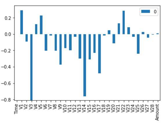
featimp = pd.Series(clf.feature_importances_,index=data_features_train.columns).sort_values(ascending=False)
print(featimp) # this is the property of Random Forest classifier that it provide us the importance 
# of the features use
 
V14                  0.206364
V10                  0.134424
V11                  0.098375
V12                  0.097194
V17                  0.088706
V4                   0.075658
V3                   0.071006
V16                  0.034599
V2                   0.020407
V18                  0.019018
V7                   0.017165
V21                  0.014312
V27                  0.011712
V19                  0.011044
V8                   0.010244
V1                   0.008564
Normalized Amount    0.007908
V9                   0.007183
V20                  0.007094
V15                  0.006852
V26                  0.006653
V5                   0.006597
V22                  0.006507
V13                  0.005839
V24                  0.005519
V28                  0.005390
V6                   0.005303
V25                  0.005210
V23                  0.005154
dtype: float64
 
  1. we can see this is showing the importance of feature for the making decision

  2. V14 is having a very good importance compare to other features

  3. Lets use only top 5 (V14,V10,V12,V17,V4) feature to predict using Random forest classifier only for 0.5 % 特征选择使用top 5特征

 
# make a new data with only class and V14
data1=data[["V14","V10","V12","V17","V4","Class"]]
data1.head()
 
 V14V10V12V17V4Class
0 -0.311169 0.090794 -0.617801 0.207971 1.378155 0
1 -0.143772 -0.166974 1.065235 -0.114805 0.448154 0
2 -0.165946 0.207643 0.066084 1.109969 0.379780 0
3 -0.287924 -0.054952 0.178228 -0.684093 -0.863291 0
4 -1.119670 0.753074 0.538196 -0.237033 0.403034 0
 
Undersample_data1 = undersample(normal_indices,fraud_indices,1)
#only for 50 % proportion it means normal transaction and fraud transaction are equal so passing 
Undersample_data1_features_train,Undersample_data1_features_test,Undersample_data1_labels_train,Undersample_data1_labels_test = data_prepration(Undersample_data1)
 
the normal transacation proportion is : 0.5
the fraud transacation proportion is : 0.5
total number of record in resampled data is: 984
length of training data
688
length of test data
296
 
clf= RandomForestClassifier(n_estimators=100)
model(clf,Undersample_data1_features_train,Undersample_data1_features_test,Undersample_data1_labels_train,Undersample_data1_labels_test)
 
the recall for this model is : 0.93006993007
TP 133
TN 149
FP 4
FN 10
----------Classification Report------------------------------------
             precision    recall  f1-score   support

          0       0.94      0.97      0.96       153
          1       0.97      0.93      0.95       143

avg / total       0.95      0.95      0.95       296

 全量数据没有测试????但从acc和recall看,top5特征的效果也还不错!!!
 

Over Sampling

 
  1. In my previous version I got the 100 recall and 98 % precision by using Random forest with the over sampled data but in real it was due to over fitting because i was taking whole fraud data and was training for that and I was doing the testing on the same data.

  2. Please find link of previous version for more understanding Link

  1. Thanks to Mr. Dominik Stuerzer for help
 
# now we will divied our data sets into two part and we will train and test and will oversample the train data and predict for test data
# lets import data again
data = pd.read_csv("../input/creditcard.csv",header = 0)
print("length of training data",len(data))
print("length of normal data",len(data[data["Class"]==0]))
print("length of fraud  data",len(data[data["Class"]==1]))
 
length of training data 284807
length of normal data 284315
length of fraud  data 492
 
data_train_X,data_test_X,data_train_y,data_test_y=data_prepration(data)
data_train_X.columns
data_train_y.columns
 
length of training data
199364
length of test data
85443
Index(['Class'], dtype='object')
 
# ok Now we have a traing data
data_train_X["Class"]= data_train_y["Class"] # combining class with original data
data_train = data_train_X.copy() # for naming conevntion
print("length of training data",len(data_train))
# Now make data set of normal transction from train data
normal_data = data_train[data_train["Class"]==0]
print("length of normal data",len(normal_data))
fraud_data = data_train[data_train["Class"]==1]
print("length of fraud data",len(fraud_data))
 
length of training data 199364
length of normal data 199009
length of fraud data 355
 
# Now start oversamoling of training data 
# means we will duplicate many times the value of fraud data #直接复制365份!!!
for i in range (365): # the number is choosen by myself on basis of nnumber of fraud transaction
    normal_data= normal_data.append(fraud_data)
os_data = normal_data.copy() 
print("length of oversampled data is ",len(os_data))
print("Number of normal transcation in oversampled data",len(os_data[os_data["Class"]==0]))
print("No.of fraud transcation",len(os_data[os_data["Class"]==1]))
print("Proportion of Normal data in oversampled data is ",len(os_data[os_data["Class"]==0])/len(os_data))
print("Proportion of fraud data in oversampled data is ",len(os_data[os_data["Class"]==1])/len(os_data))
 
length of oversampled data is  328584
Number of normal transcation in oversampled data 199009
No.of fraud transcation 129575
Proportion of Normal data in oversampled data is  0.6056563922771651
Proportion of fraud data in oversampled data is  0.39434360772283494
 
  1. The proportion now becomes the 60 % and 40 % that is good now
 
# before applying any model standerdize our data amount 
os_data["Normalized Amount"] = StandardScaler().fit_transform(os_data['Amount'].reshape(-1, 1))
os_data.drop(["Time","Amount"],axis=1,inplace=True) 其实随机森林对特征是否标准化无感,但是svm和LR就非常非常关键了
os_data.head()
 
 V1V2V3V4V5V6V7V8V9V10...V21V22V23V24V25V26V27V28ClassNormalized Amount
82656 1.356574 -1.535896 1.014585 -0.980949 -1.840651 0.495094 -1.535552 0.235415 -0.847601 1.180545 ... -0.578444 -0.948479 0.038288 -0.051798 0.350549 -0.338308 0.073518 0.017247 0 -0.240655
202761 0.078384 0.693709 -0.282273 -1.007720 1.058216 -0.035670 0.838345 0.070423 -0.094317 -0.221217 ... -0.303203 -0.775385 -0.086534 -1.414806 -0.360046 0.208073 0.234031 0.072388 0 -0.371265
85985 -3.549282 -3.403880 2.389801 1.080311 1.683676 -1.100104 -0.699287 0.171644 0.935805 -0.256182 ... -0.284722 0.428109 2.844650 0.006528 0.466552 0.421108 0.260494 -0.472237 0 -0.383217
215180 2.084961 0.009129 -3.842413 -0.551511 3.139773 2.743495 0.130580 0.552759 -0.030368 -0.295843 ... 0.034740 0.187883 -0.014668 0.682901 0.410981 0.734260 -0.081080 -0.064606 0 -0.374769
75855 1.193268 -0.071682 0.611175 -0.232721 -0.478724 -0.216029 -0.329775 0.071921 0.009225 -0.112748 ... -0.043944 -0.080370 0.101692 0.090155 0.041104 0.914386 -0.053130 -0.002135 0 -0.388278

5 rows × 30 columns

 
# Now use this oversampled data for trainig the model and predict value for the test data that we created before
# now let us try within the the oversampled data itself
# for that we need to split our oversampled data into train and test
# so call our function data Prepration with oversampled data
os_train_X,os_test_X,os_train_y,os_test_y=data_prepration(os_data)
clf= RandomForestClassifier(n_estimators=100)
model(clf,os_train_X,os_test_X,os_train_y,os_test_y)
 
length of training data
230008
length of test data
98576
the recall for this model is : 1.0
TP 38975
TN 59596
FP 5
FN 0
----------Classification Report------------------------------------
             precision    recall  f1-score   support

          0       1.00      1.00      1.00     59601
          1       1.00      1.00      1.00     38975

avg / total       1.00      1.00      1.00     98576


Observations

  1. As it have too many sample of same fraud data so may be the all which are present in train data are present in test data also so we can say it is over fitting #重复样本太多,过拟合严重
  2. So lets try with test data that one which we created in starting of oversampling segment no fraud transaction from that data have been repeated here #在过采样前先拿出一点数据出来做测试,而不是过采样之后!!!
  3. Lets try
 
# now take all over sampled data as trainging and test it for test data
os_data_X = os_data.ix[:,os_data.columns != "Class"]
os_data_y = os_data.ix[:,os_data.columns == "Class"]
#for that we have to standrdize the normal amount and drop the time from it
data_test_X["Normalized Amount"] = StandardScaler().fit_transform(data_test_X['Amount'].reshape(-1, 1))
data_test_X.drop(["Time","Amount"],axis=1,inplace=True)
data_test_X.head()
 
 V1V2V3V4V5V6V7V8V9V10...V20V21V22V23V24V25V26V27V28Normalized Amount
11514 1.451038 -0.603389 0.007125 -0.616909 -0.260790 0.474328 -0.826944 0.042607 1.101926 0.110945 ... -0.054708 -0.249080 -0.389480 -0.151185 -1.380077 0.610950 -0.163068 -0.005513 -0.013058 -0.320476
162269 -6.697569 4.179960 -4.866476 -0.626586 -3.024024 -1.324855 -0.835983 2.692196 1.844012 2.825418 ... 0.649757 0.035932 0.852066 0.245004 1.155756 0.098178 -0.214949 0.996161 1.252345 0.050478
158202 2.104037 0.065442 -1.428655 0.323540 0.393572 -0.720375 0.054806 -0.347347 2.082360 -0.464191 ... -0.271997 0.093486 0.657963 -0.007259 0.431328 0.360900 -0.474799 -0.024631 -0.056532 -0.357576
203014 -2.602873 -1.593223 0.029747 -3.264885 1.156256 0.930955 -0.477817 0.828043 -0.543710 -0.592860 ... -1.154639 -0.680829 -1.305820 0.841971 -1.009959 -0.495993 0.056765 -0.434924 0.375225 -0.176200
129141 -1.325968 1.418993 -0.531978 -1.422122 2.635501 3.223994 0.477654 0.538505 0.756693 1.527077 ... 0.941600 -0.599390 -1.053070 -0.004289 0.917391 0.221693 0.059054 0.459664 -0.018905 -0.324681

5 rows × 29 columns

 
# now use it for modeling
clf= RandomForestClassifier(n_estimators=100)
model(clf,os_data_X,data_test_X,os_data_y,data_test_y)
 
the recall for this model is : 0.773722627737
TP 106
TN 85300
FP 6
FN 31
----------Classification Report------------------------------------
             precision    recall  f1-score   support

          0       1.00      1.00      1.00     85306
          1       0.95      0.77      0.85       137

avg / total       1.00      1.00      1.00     85443


Observations

  1. Now here we can see recall decrease to only 83 % which is not bad but not good also
  2. The precision is 0.93 which is good
  3. from these observation we can say that the oversampling is better than the Under sampling because on Under sampling we were loosing a large amount of data or we can say a good amount of information so why the there precision was very low
 

SMOTE

 
# Lets Use SMOTE for Sampling
# As I mentioned it is also a type of oversampling but in this the data is not replicated but they are created 
#lets start with importing libraries
from imblearn.over_sampling import SMOTE
data = pd.read_csv('../input/creditcard.csv')
 
os = SMOTE(random_state=0) #   We are using SMOTE as the function for oversampling
# now we can devided our data into training and test data
# Call our method data prepration on our dataset
data_train_X,data_test_X,data_train_y,data_test_y=data_prepration(data)
columns = data_train_X.columns
 
length of training data
199364
length of test data
85443
 
# now use SMOTE to oversample our train data which have features data_train_X and labels in data_train_y
os_data_X,os_data_y=os.fit_sample(data_train_X,data_train_y)
os_data_X = pd.DataFrame(data=os_data_X,columns=columns )
os_data_y= pd.DataFrame(data=os_data_y,columns=["Class"])
# we can Check the numbers of our data
print("length of oversampled data is ",len(os_data_X))
print("Number of normal transcation in oversampled data",len(os_data_y[os_data_y["Class"]==0]))
print("No.of fraud transcation",len(os_data_y[os_data_y["Class"]==1]))
print("Proportion of Normal data in oversampled data is ",len(os_data_y[os_data_y["Class"]==0])/len(os_data_X))
print("Proportion of fraud data in oversampled data is ",len(os_data_y[os_data_y["Class"]==1])/len(os_data_X))
 
length of oversampled data is  398078
Number of normal transcation in oversampled data 199039
No.of fraud transcation 199039 # smote后1:1了
Proportion of Normal data in oversampled data is  0.5
Proportion of fraud data in oversampled data is  0.5
 
  1. By using Smote we are getting a 50 - 50 each

  2. No need of checking here in over sampled data itself from previous we know it will be overfitting

  3. let us check with the test data direct

 
# Let us first do our amount normalised and other that we are doing above  #过采样前一定一定要标准化!!!
os_data_X["Normalized Amount"] = StandardScaler().fit_transform(os_data_X['Amount'].reshape(-1, 1))
os_data_X.drop(["Time","Amount"],axis=1,inplace=True)
data_test_X["Normalized Amount"] = StandardScaler().fit_transform(data_test_X['Amount'].reshape(-1, 1))
data_test_X.drop(["Time","Amount"],axis=1,inplace=True)
 
# Now start modeling
clf= RandomForestClassifier(n_estimators=100)
# train data using oversampled data and predict for the test data
model(clf,os_data_X,data_test_X,os_data_y,data_test_y)
 
the recall for this model is : 0.862275449102
TP 144
TN 85253
FP 23
FN 23
----------Classification Report------------------------------------
             precision    recall  f1-score   support

          0       1.00      1.00      1.00     85276
          1       0.86      0.86      0.86       167

avg / total       1.00      1.00      1.00     85443


observation

  1. The recall is nearby the previous one done by over sampling
  2. The precision decrease in this case

综合结论就是:随机森林+过采样(直接复制或者smote后,黑白比例1:3)效果比较好!

from:http://www.dataguru.cn/article-11449-1.html

用Python作信用卡欺诈预测 ——欠采样、效果不好

一、项目简介
Credit Card Fraud Detection
https://www.kaggle.com/dalpozz/creditcardfraud
是一个典型的分类问题,欺诈分类的比例比较小,直接使用分类模型容易忽略。在实际应用场景下往往是保证一定准确率的情况下尽量提高召回率。一个典型案例是汽车制造行业,一旦发生一例汽车安全故障,同批次的车辆需要全部召回,造成了巨大的经济损失。
 
二、数据印象
2.1. 简单数据分析
数据规模:中度规模(对于mac而言)。数据共284807条,后期算法选择需要注意复杂度。
 
数据特征:V1~V28是PCA的结果,而且进行了规范化,可以做一些统计上的特征学习;Amount字段和Time字段可以进行额外的统计学和bucket统计。
数据质量:无缺失值,数据规整,享受啊。
经验:时间字段较好可以处理为月份、小时和日期,直接的秒数字段往往无意义。
 
2.2. 探索性数据分析
 
三、数据预处理
数据已经十分规整了,所以先直接使用基础模型来预测下数据。
 
 
L1规划化
L1规范化的模型
 
L2规范化
L2规范化的模型
Baseline基础模型:采用线性模型,利用L1的稀疏性,precision和recall均可以达到0.85左右,roc_auc可以达到0.79左右。
基础模型结果
 
由上图可见:
precision较大时波动波动比较大。recall大于0.8后,准确率下滑严重。
AUC面积是0.97,后来根据参考文献3知,AUC大于0.92时之后比较难修正。
Baseline模型的评价metric:
收集更多的数据,不适合这个场景。
改变评价标准:
使用混淆矩阵计算准确度和回收度。
F1score
Kappa
ROC curves - sensitivity/specificity ratio
 
数据采样处理
- 收集等多数据:不适合这个场景。- 过采样Over-sampling:当数据集较少时,主动添加少类别的数据;
 SMOT算法通过插值来实现。不适合本数据集。容易过拟合,运算时间长。- 欠采样Under-sampling:
 当数据集足够大时,删除大类别的数据;集成方法`EasyEnsemble/BalanceCascade`
 通过将反例放在不同学习器中使用,从全局看不会丢失重要信息。
本案例数据量中等:选用欠采样+EasyEnsemble的方式进行数据处理。
 
使用im-balanced生成测试数据。
http://contrib.scikit-learn.org/imbalanced-learn/auto_examples/index.html
 
from imblearn.ensemble import EasyEnsemblen_subsets = X.size * 2 / 
(us_X.size) - 1ee = EasyEnsemble(n_subsets=n_subsets)sample_X, 
sample_y = ee.fit_sample(X, y)
 
四、模型印象
模型:
选用easy_ensemble模型来优化。
具体实现代码见在线脚本
 
核心adboost代码如下:
 
 
结果如下:
 
easy_ensembel
对比普通的adboost数据
对比图
由上图可知,easy_ensemble提升了平滑度,但是AUC未有提升。
 
五、特征选择和特征学习
L1模型进行了嵌入式的特征选择,效果优于L2模型。在寻找解释性时会有帮助。
根据数据的统计特征,可以学习一些统计变量。
统计学习
增加如下的特征。
 
 
六、分析结果
使用SNE分析(常用于非线性可视化分析)来观看一次under_sample的结果。
https://bindog.github.io/blog/2016/06/04/from-sne-to-tsne-to-largevis/
 
如下图所示
SNE图
由上图可知两种类别的数据是可以区分的,但是部分数据融合在一起,当追求recall较大时,将会误判大量数据。
 
七、迭代问题
可以优化的方向:
可以通过学习新的特征,将数据在新维度上拉开距离
在计算机能力允许的情况下,设置合适的round轮次来调参。
 
八、表述模型
根据模型的SNE图和数据性可知,数据质量是比较好的。
easy_ensemble模型本身使用了adboost和bagging,每棵tree的复杂度不高,降低了bias;通过bagging,降低了variance。最终得到了较好的P-R图和AUC值。
通过LR模型的稀疏性特征值,可以制作出一个解释性报告。
 
参考
GBM vs xgboost vs lightGBM
https://www.kaggle.com/nschneider/gbm-vs-xgboost-vs-lightgbm
 
imbalanced-learn
http://contrib.scikit-learn.org/imbalanced-learn/index.html
 
Exploratory Undersampling for Class-Imbalance Learning
https://cs.nju.edu.cn/zhouzh/zhouzh.files/publication/tsmcb09.pdf
原文地址:https://www.cnblogs.com/bonelee/p/9087286.html