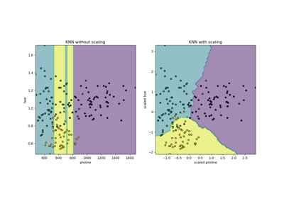
RESCALING attribute data to values to scale the range in [0, 1] or [−1, 1] is useful for the optimization algorithms, such as gradient descent, that are used within machine learning algorithms that weight inputs (e.g. regression and neural networks). Rescaling is also used for algorithms that use distance measurements for example K-Nearest-Neighbors (KNN). Rescaling like this is sometimes called "normalization". MinMaxScaler class in python skikit-learn does this.
NORMALIZING attribute data is used to rescale components of a feature vector to have the complete vector length of 1. This is "scaling by unit length". This usually means dividing each component of the feature vector by the Euclidiean length of the vector but can also be Manhattan or other distance measurements. This pre-processing rescaling method is useful for sparse attribute features and algorithms using distance to learn such as KNN. Python scikit-learn Normalizer class can be used for this.
STANDARDIZING attribute data is also a preprocessing method but it assumes a Gaussian distribution of input features. It "standardizes" to a mean of 0 and a standard deviation of 1. This works better with linear regression, logistic regression and linear discriminate analysis. Python StandardScaler class in scikit-learn works for this.
from:skearn DOC:
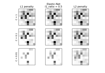
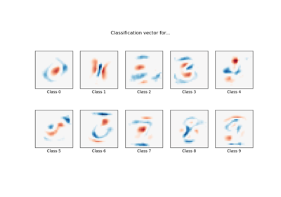
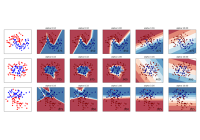
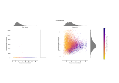
Examples using sklearn.preprocessing.StandardScaler
from:https://www.programcreek.com/python/example/82501/sklearn.preprocessing.MinMaxScaler-----maybe svm is wrong!
Python sklearn.preprocessing.MinMaxScaler() Examples
The following are 50 code examples for showing how to use sklearn.preprocessing.MinMaxScaler(). They are extracted from open source Python projects. You can vote up the examples you like or vote down the exmaples you don't like. You can also save this page to your account.
| Project: sef Author: passalis File: classification.py View Source Project | 7 votes | |
def evaluate_svm(train_data, train_labels, test_data, test_labels, n_jobs=-1):
    """
    Evaluates a representation using a Linear SVM
    It uses 3-fold cross validation for selecting the C parameter
    :param train_data:
    :param train_labels:
    :param test_data:
    :param test_labels:
    :param n_jobs:
    :return: the test accuracy
    """

    # Scale data to 0-1
    scaler = MinMaxScaler()
    train_data = scaler.fit_transform(train_data)
    test_data = scaler.transform(test_data)

    parameters = {'kernel': ['linear'], 'C': [0.0001, 0.001, 0.01, 0.1, 1, 10, 100, 1000, 10000, 100000]}
    model = svm.SVC(max_iter=10000)
    clf = grid_search.GridSearchCV(model, parameters, n_jobs=n_jobs, cv=3)
    clf.fit(train_data, train_labels)
    lin_svm_test = clf.score(test_data, test_labels)
    return lin_svm_test
| Project: golden_touch Author: at553 File: predict.py View Source Project | 6 votes | |
def train_model(self):
        # scale
        scaler = MinMaxScaler(feature_range=(0, 1))
        dataset = scaler.fit_transform(self.data)

        # split into train and test sets
        train_size = int(len(dataset) * 0.95)
        train, test = dataset[0:train_size, :], dataset[train_size:len(dataset), :]

        look_back = 5
        trainX, trainY = self.create_dataset(train, look_back)

        # reshape input to be [samples, time steps, features]
        trainX = numpy.reshape(trainX, (trainX.shape[0], 1, trainX.shape[1]))
        # create and fit the LSTM network
        model = Sequential()
        model.add(LSTM(6, input_dim=look_back))
        model.add(Dense(1))
        model.compile(loss='mean_squared_error', optimizer='adam')
        model.fit(trainX, trainY, nb_epoch=100, batch_size=1, verbose=2)
        return model
官方的dbscan聚类使用 StandardScaler
http://scikit-learn.org/stable/auto_examples/cluster/plot_dbscan.html#example-cluster-plot-dbscan-py
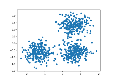
Demo of DBSCAN clustering algorithm
Finds core samples of high density and expands clusters from them.
Out:
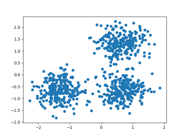
Estimated number of clusters: 3
Homogeneity: 0.953
Completeness: 0.883
V-measure: 0.917
Adjusted Rand Index: 0.952
Adjusted Mutual Information: 0.883
Silhouette Coefficient: 0.626
print(__doc__)

import numpy as np

from sklearn.cluster import DBSCAN
from sklearn import metrics
from sklearn.datasets.samples_generator import make_blobs
from sklearn.preprocessing import StandardScaler


# #############################################################################
# Generate sample data
centers = [[1, 1], [-1, -1], [1, -1]]
X, labels_true = make_blobs(n_samples=750, centers=centers, cluster_std=0.4,
                            random_state=0)

X = StandardScaler().fit_transform(X)

# #############################################################################
# Compute DBSCAN
db = DBSCAN(eps=0.3, min_samples=10).fit(X)
core_samples_mask = np.zeros_like(db.labels_, dtype=bool)
core_samples_mask[db.core_sample_indices_] = True
labels = db.labels_

# Number of clusters in labels, ignoring noise if present.
n_clusters_ = len(set(labels)) - (1 if -1 in labels else 0)

print('Estimated number of clusters: %d' % n_clusters_)
print("Homogeneity: %0.3f" % metrics.homogeneity_score(labels_true, labels))
print("Completeness: %0.3f" % metrics.completeness_score(labels_true, labels))
print("V-measure: %0.3f" % metrics.v_measure_score(labels_true, labels))
print("Adjusted Rand Index: %0.3f"
      % metrics.adjusted_rand_score(labels_true, labels))
print("Adjusted Mutual Information: %0.3f"
      % metrics.adjusted_mutual_info_score(labels_true, labels))
print("Silhouette Coefficient: %0.3f"
      % metrics.silhouette_score(X, labels))

# #############################################################################
# Plot result
import matplotlib.pyplot as plt

# Black removed and is used for noise instead.
unique_labels = set(labels)
colors = [plt.cm.Spectral(each)
          for each in np.linspace(0, 1, len(unique_labels))]
for k, col in zip(unique_labels, colors):
    if k == -1:
        # Black used for noise.
        col = [0, 0, 0, 1]

    class_member_mask = (labels == k)

    xy = X[class_member_mask & core_samples_mask]
    plt.plot(xy[:, 0], xy[:, 1], 'o', markerfacecolor=tuple(col),
             markeredgecolor='k', markersize=14)

    xy = X[class_member_mask & ~core_samples_mask]
    plt.plot(xy[:, 0], xy[:, 1], 'o', markerfacecolor=tuple(col),
             markeredgecolor='k', markersize=6)

plt.title('Estimated number of clusters: %d' % n_clusters_)
plt.show()
https://chrisalbon.com/machine_learning/clustering/k-means_clustering/ 这里的iris聚类也用到了
k-Means Clustering

Preliminaries
# Load libraries
from sklearn import datasets
from sklearn.preprocessing import StandardScaler
from sklearn.cluster import KMeans
Load Iris Flower Dataset
# Load data
iris = datasets.load_iris()
X = iris.data
Standardize Features
# Standarize features
scaler = StandardScaler()
X_std = scaler.fit_transform(X)
Conduct k-Means Clustering
# Create k-mean object
clt = KMeans(n_clusters=3, random_state=0, n_jobs=-1)

# Train model
model = clt.fit(X_std)
Show Each Observation’s Cluster Membership
# View predict class
model.labels_
array([1, 1, 1, 1, 1, 1, 1, 1, 1, 1, 1, 1, 1, 1, 1, 1, 1, 1, 1, 1, 1, 1, 1,
1, 1, 1, 1, 1, 1, 1, 1, 1, 1, 1, 1, 1, 1, 1, 1, 1, 1, 1, 1, 1, 1, 1,
1, 1, 1, 1, 0, 0, 0, 2, 2, 2, 0, 2, 2, 2, 2, 2, 2, 2, 2, 0, 2, 2, 2,
2, 0, 2, 2, 2, 2, 0, 0, 0, 2, 2, 2, 2, 2, 2, 2, 0, 0, 2, 2, 2, 2, 2,
2, 2, 2, 2, 2, 2, 2, 2, 0, 2, 0, 0, 0, 0, 2, 0, 0, 0, 0, 0, 0, 2, 2,
0, 0, 0, 0, 2, 0, 2, 0, 2, 0, 0, 2, 0, 0, 0, 0, 0, 0, 2, 2, 0, 0, 0,
2, 0, 0, 0, 2, 0, 0, 0, 2, 0, 0, 2], dtype=int32)
Create New Observation
# Create new observation
new_observation = [[0.8, 0.8, 0.8, 0.8]]
Predict Observation’s Cluster
# Predict observation's cluster
model.predict(new_observation)
array([0], dtype=int32)
View Centers Of Each Cluster
# View cluster centers
model.cluster_centers_
array([[ 1.13597027, 0.09659843, 0.996271 , 1.01717187],
[-1.01457897, 0.84230679, -1.30487835, -1.25512862],
[-0.05021989, -0.88029181, 0.34753171, 0.28206327]])
详细见:详见http://d0evi1.com/sklearn/preprocessing/
标准化
变换后各维特征有0均值,单位方差。也叫z-score规范化(零均值规范化)。计算方式是将特征值减去均值,除以标准差。
from sklearn.preprocessing import scaleX = np.array([[ 1., -1., 2.],[ 2., 0., 0.],[ 0., 1., -1.]])scale(X)
一般会把train和test集放在一起做标准化,或者在train集上做标准化后,用同样的标准化器去标准化test集,此时可以用scaler
from sklearn.preprocessing import StandardScalerscaler = StandardScaler().fit(train)scaler.transform(train)scaler.transform(test)
最小-最大规范化
最小-最大规范化对原始数据进行线性变换,变换到[0,1]区间(也可以是其他固定最小最大值的区间)
min_max_scaler = sklearn.preprocessing.MinMaxScaler()min_max_scaler.fit_transform(X_train)
规范化:正则化
规范化是将不同变化范围的值映射到相同的固定范围,常见的是[0,1],此时也称为归一化。《机器学习》周志华
X = [[ 1, -1, 2],[ 2, 0, 0], [ 0, 1, -1]]sklearn.preprocessing.normalize(X, norm='l2')
array([[ 0.40, -0.40, 0.81], [ 1, 0, 0], [ 0, 0.70, -0.70]])
可以发现对于每一个样本都有,0.4^2+0.4^2+0.81^2=1,这就是L2 norm,变换后每个样本的各维特征的平方和为1。类似地,L1 norm则是变换后每个样本的各维特征的绝对值和为1。还有max norm,则是将每个样本的各维特征除以该样本各维特征的最大值。
在度量样本之间相似性时,如果使用的是二次型kernel,需要做Normalization
特征二值化
给定阈值,将特征转换为0/1
binarizer = sklearn.preprocessing.Binarizer(threshold=1.1)binarizer.transform(X)
标签二值化
from sklearn import preprocessinglb = preprocessing.LabelBinarizer()lb.fit([1, 2, 6, 4, 2])lb.classes_array([1, 2, 4, 6])lb.transform([1, 6])#必须[1, 2, 6, 4, 2]里面array([[1, 0, 0, 0],[0, 0, 0, 1]])
类别特征编码
标签编码
含有异常值
sklearn.preprocessing.robust_scale
生成多项式
原始特征

转化后

poly = sklearn.preprocessing.PolynomialFeatures(2)poly.fit_transform(X)
http://shujuren.org/article/234.html
一、标准化(Z-Score),或者去除均值和方差缩放
公式为:(X-mean)/std 计算时对每个属性/每列分别进行。
将数据按期属性(按列进行)减去其均值,并处以其方差。得到的结果是,对于每个属性/每列来说所有数据都聚集在0附近,方差为1。
实现时,有两种不同的方式:
-
使用sklearn.preprocessing.scale()函数,可以直接将给定数据进行标准化。
|
1
2
3
4
5
6
7
8
9
10
11
12
13
14
15
16
17
18
|
>>> from sklearn import preprocessing>>> import numpy as np>>> X = np.array([[ 1., -1., 2.],... [ 2., 0., 0.],... [ 0., 1., -1.]])>>> X_scaled = preprocessing.scale(X)>>> X_scaled array([[ 0. ..., -1.22..., 1.33...], [ 1.22..., 0. ..., -0.26...], [-1.22..., 1.22..., -1.06...]])>>>#处理后数据的均值和方差>>> X_scaled.mean(axis=0)array([ 0., 0., 0.])>>> X_scaled.std(axis=0)array([ 1., 1., 1.]) |
-
使用sklearn.preprocessing.StandardScaler类,使用该类的好处在于可以保存训练集中的参数(均值、方差)直接使用其对象转换测试集数据。
|
1
2
3
4
5
6
7
8
9
10
11
12
13
14
15
16
17
18
19
|
>>> scaler = preprocessing.StandardScaler().fit(X)>>> scalerStandardScaler(copy=True, with_mean=True, with_std=True)>>> scaler.mean_ array([ 1. ..., 0. ..., 0.33...])>>> scaler.std_ array([ 0.81..., 0.81..., 1.24...])>>> scaler.transform(X) array([[ 0. ..., -1.22..., 1.33...], [ 1.22..., 0. ..., -0.26...], [-1.22..., 1.22..., -1.06...]])>>>#可以直接使用训练集对测试集数据进行转换>>> scaler.transform([[-1., 1., 0.]]) array([[-2.44..., 1.22..., -0.26...]]) |
二、将属性缩放到一个指定范围
除了上述介绍的方法之外,另一种常用的方法是将属性缩放到一个指定的最大和最小值(通常是1-0)之间,这可以通过preprocessing.MinMaxScaler类实现。
使用这种方法的目的包括:
1、对于方差非常小的属性可以增强其稳定性。
2、维持稀疏矩阵中为0的条目。
|
1
2
3
4
5
6
7
8
9
10
11
12
13
14
15
16
17
18
19
20
21
22
23
24
|
>>> X_train = np.array([[ 1., -1., 2.],... [ 2., 0., 0.],... [ 0., 1., -1.]])...>>> min_max_scaler = preprocessing.MinMaxScaler()>>> X_train_minmax = min_max_scaler.fit_transform(X_train)>>> X_train_minmaxarray([[ 0.5 , 0. , 1. ], [ 1. , 0.5 , 0.33333333], [ 0. , 1. , 0. ]])>>> #将相同的缩放应用到测试集数据中>>> X_test = np.array([[ -3., -1., 4.]])>>> X_test_minmax = min_max_scaler.transform(X_test)>>> X_test_minmaxarray([[-1.5 , 0. , 1.66666667]])>>> #缩放因子等属性>>> min_max_scaler.scale_ array([ 0.5 , 0.5 , 0.33...])>>> min_max_scaler.min_ array([ 0. , 0.5 , 0.33...]) |
当然,在构造类对象的时候也可以直接指定最大最小值的范围:feature_range=(min, max),此时应用的公式变为:
X_std=(X-X.min(axis=0))/(X.max(axis=0)-X.min(axis=0))
X_scaled=X_std/(max-min)+min
三、正则化(Normalization)
正则化的过程是将每个样本缩放到单位范数(每个样本的范数为1),如果后面要使用如二次型(点积)或者其它核方法计算两个样本之间的相似性这个方法会很有用。
Normalization主要思想是对每个样本计算其p-范数,然后对该样本中每个元素除以该范数,这样处理的结果是使得每个处理后样本的p-范数(l1-norm,l2-norm)等于1。
该方法主要应用于文本分类和聚类中。例如,对于两个TF-IDF向量的l2-norm进行点积,就可以得到这两个向量的余弦相似性。
1、可以使用preprocessing.normalize()函数对指定数据进行转换:
|
1
2
3
4
5
6
7
8
9
|
>>> X = [[ 1., -1., 2.],... [ 2., 0., 0.],... [ 0., 1., -1.]]>>> X_normalized = preprocessing.normalize(X, norm='l2')>>> X_normalized array([[ 0.40..., -0.40..., 0.81...], [ 1. ..., 0. ..., 0. ...], [ 0. ..., 0.70..., -0.70...]]) |
2、可以使用processing.Normalizer()类实现对训练集和测试集的拟合和转换:
|
1
2
3
4
5
6
7
8
9
10
11
12
|
>>> normalizer = preprocessing.Normalizer().fit(X) # fit does nothing>>> normalizerNormalizer(copy=True, norm='l2')>>>>>> normalizer.transform(X) array([[ 0.40..., -0.40..., 0.81...], [ 1. ..., 0. ..., 0. ...], [ 0. ..., 0.70..., -0.70...]])>>> normalizer.transform([[-1., 1., 0.]]) array([[-0.70..., 0.70..., 0. ...]]) |
补充:
