Composite Partitioning

Ideal for both historical data and data placement
Provides high availability and manageability,like range partitioning
Improves performance for parallel DML and supports partition-wise joins
Allows more granular partition elimination
Supports composite local indexes
Does not support composite global indexes

Partitioned Indexes

Local Partitioned Indexes

Global NonPartitioned Indexes

Global Partitioned Indexes

oracle recommend:OLAP系统使用local partition index,OLTP系统使用Global partition index

local partition index易管理，一个表分区对应一个索引分区.

global partition index相对难管理一些，一个索引分区对应多个表分区.

create partition table range2, range type

CREATE TABLE  range2
(
        a int,
        b int,
        data char(20)
)
PARTITION BY RANGE(a)
(
        PARTITION p1 VALUES LESS THAN(2) tablespace TS1,
        PARTITION p2 VALUES LESS THAN(3) tablespace TS2
);

create local index for range2

CREATE INDEX local_idx1 ON RANGE2(a,b) LOCAL;

创建no-partition global index

创建GLOBAL NON PARTITION INDEX

CREATE INDEX G_IDX1 ON RANGE2(data);

--创建GLOBAL PARTATION INDEX

CREATE INDEX GP_IDX ON RANGE2(b) GLOBAL
PARTITION BY RANGE(b)
(
        PARTITION idx1 VALUES LESS THAN (1000),
        PARTITION idx2 VALUES LESS THAN (MAXVALUE)
);

--往表中灌数据
INSERT INTO range2
SELECT mod(rownum -1,2)+1,rownum,'x' FROM all_objects;

commit;

--执行分析
BEGIN
        DBMS_STATS.GATHER_TABLE_STATS('U3','RANGE2',CASCADE=>TRUE);
END;

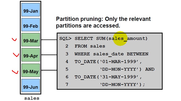
Partition Pruning(核心思想，就是只查询相关的分区表，其他无关的分区表将会智能过滤掉.提高几个数量级的查询速度)

实验一

SQL> SELECT * FROM range2 WHERE a=1 and b=1;

         A          B DATA
---------- ---------- --------------------
         1          1 x
         1          1 x
         1          1 x
         1          1 x

SQL> delete from plan_table;

0 rows deleted.

SQL> explain plan for SELECT * FROM range2 WHERE a=1 and b=1;

Explained.

SQL> set linesize 1000
SQL> select * from table(dbms_xplan.display);

PLAN_TABLE_OUTPUT
------------------------------------------------------------------------------------------------------------------------------------------------------------------------------------------------------------------------------------------------------------------------------------------------------------
Plan hash value: 370859827

-----------------------------------------------------------------------------------------------------------------
| Id  | Operation                          | Name       | Rows  | Bytes | Cost (%CPU)| Time     | Pstart| Pstop |
-----------------------------------------------------------------------------------------------------------------
|   0 | SELECT STATEMENT                   |            |     4 |   116 |     5   (0)| 00:00:01 |       |       |
|   1 |  PARTITION RANGE SINGLE            |            |     4 |   116 |     5   (0)| 00:00:01 |     1 |     1 |
|   2 |   TABLE ACCESS BY LOCAL INDEX ROWID| RANGE2     |     4 |   116 |     5   (0)| 00:00:01 |     1 |     1 |
|*  3 |    INDEX RANGE SCAN                | LOCAL_IDX1 |     4 |       |     1   (0)| 00:00:01 |     1 |     1 |
-----------------------------------------------------------------------------------------------------------------

Predicate Information (identified by operation id):
---------------------------------------------------

   3 - access("A"=1 AND "B"=1)

15 rows selected.

解析：

SELECT * FROM range2 WHERE a=1 and b=1;执行查询语句之后，通过dbms_stats.gather_table_stats执行后发现，oracle智能的过滤掉不用的分区，只从Pstart=1，到Pstop=1分区内查询，其他分区都不会去过滤.大大提供性能.下面的实验也是如此道理.

SQL> select * from range2 where a=2 and b=2;

         A          B DATA
---------- ---------- --------------------
         2          2 x
         2          2 x
         2          2 x
         2          2 x

SQL> delete from plan_table;

4 rows deleted.

SQL> explain plan for select * from range2 where a=2 and b=2;

Explained.

SQL> select * from table(dbms_xplan.display);

PLAN_TABLE_OUTPUT
------------------------------------------------------------------------------------------------------------------------------------------------------------------------------------------------------------------------------------------------------------------------------------------------------------
Plan hash value: 370859827

-----------------------------------------------------------------------------------------------------------------
| Id  | Operation                          | Name       | Rows  | Bytes | Cost (%CPU)| Time     | Pstart| Pstop |
-----------------------------------------------------------------------------------------------------------------
|   0 | SELECT STATEMENT                   |            |     4 |   116 |     5   (0)| 00:00:01 |       |       |
|   1 |  PARTITION RANGE SINGLE            |            |     4 |   116 |     5   (0)| 00:00:01 |     2 |     2 |
|   2 |   TABLE ACCESS BY LOCAL INDEX ROWID| RANGE2     |     4 |   116 |     5   (0)| 00:00:01 |     2 |     2 |
|*  3 |    INDEX RANGE SCAN                | LOCAL_IDX1 |     4 |       |     1   (0)| 00:00:01 |     2 |     2 |
-----------------------------------------------------------------------------------------------------------------

Predicate Information (identified by operation id):
---------------------------------------------------

   3 - access("A"=2 AND "B"=2)

15 rows selected.

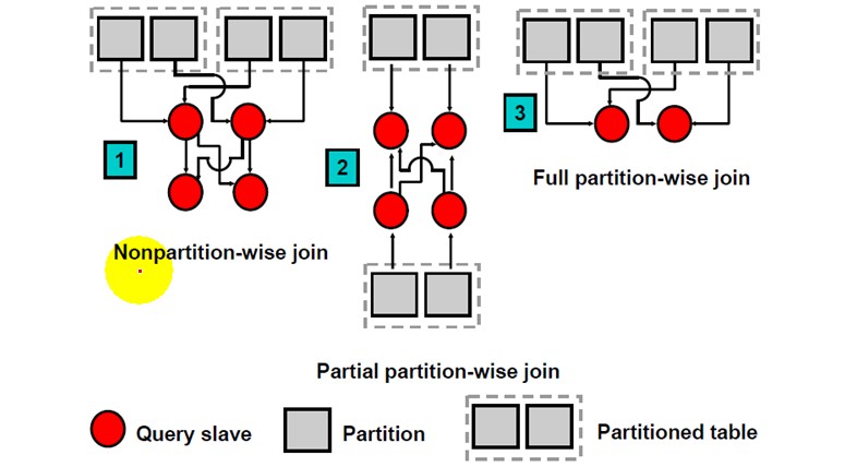
Partition-wise join(在进行Join的时候，能够智能的意识到哪些分区参与Join，哪些分区不参与)

Statistics Collection

You can gather object-,partition-,or subpartition level statistics.
There are GLOBAL or NON-GLOBAL statistics.
The dbms_stats package can gahter global statistics at any level for tables only.
It is not possible to gather:
- -Global histograms
- -Global statistics for indexes

Summary

In this lesson,you should have learned how to do the following:

Compare and evaluate the different storage structures
Examine different data access method
Implement different partitioning mehtods